PyCon US 2026
Breaking the Speed Limit
Statistician’s workflow. Fast models.
Wenxin Jiang, Jian Yin | Biostatistics, CityU HK
Target first. Speed later. Preserve statistical results.
Simulate for control. Define baseline behavior.
Python orchestrates execution. Match tools to bottlenecks.
Welcome everyone. I am Wenxin, And this is my colleague Jian. We are PhD students at City University of Hong Kong. Our research focuses on developing statistical methods and software for large-scale genetic data analysis. But, fortunately, we are not here to talk about genetics or mathematics. Today, we are discussing how to safely push the speed limits of statistical models in Python.
In fields like genetics, speed is absolutely critical. The human genome has millions of variants. When we test their relationships to a disease, we execute billions of calculations. Without optimization, a single experiment can take months. If we can speed up the code by 10x, we can get results in several days.
So, we must write fast code. But there is a strict rule: we cannot sacrifice statistical validity. If an optimized engine slightly changes the math, we are simply producing the wrong scientific conclusion faster.
Today, we will explore how to prevent that.
Why this talk
Speed follows validation
Specify. Execute. Verify.
Target First Define core statistic.
Executable Reference Build matchable baseline.
Conditional Speed Answer identical question.
Speed only counts when the math is preserved.
The governing rule of this framework is: Speed follows validation.
Usually, we start with a baseline implementation that directly translates our mathematical formula into code. This code is often not optimized, but it serves as a reference. We then validate that this code produces the correct or expected results, often using simulation. Only after we have established that the baseline code is correct do we consider optimizing it for speed.
Simulation as testing
Simulation creates an answer key
Real-world data doesn't have ground truth.
01
Statistical target
What to estimate?
02
Simulation scenarios
Edge cases. Nulls.
03
Reference implementation
Executable baseline.
validate before timing
04
Validation checks
Prove equivalence.
05
Bottleneck shape
Identify the limit.
06
Acceleration
Apply smallest tool.
→
→
→
→
Because real-world data does not have ground truth, if we simply run our code on it and we cannot check if the results are correct. Instead, we use simulation to create synthetic datasets where we know the underlying parameters and relationships. By designing simulation scenarios, we can ensure that our implementation behaves correctly across a range of inputs. This allows us to test whether our accelerated code is producing the correct results compared to the known truth and to our baseline implementation.
This process of validating before timing ensures that we are optimizing code that is already correct, rather than optimizing code that may have bugs. Also, by using simulation, we can identify the bottleneck shapes in our code, which informs us on how to apply the appropriate optimization techniques.
Programmer bridge
Simulation turns statistical behavior into tests
Expected behavior is statistical.
How simulation maps to software testing
Unit tests
Fixed-seed equivalence.
Property tests
Null invariants. Calibration.
Stress tests
Outliers. High dimension.
Load tests
Scale samples. Scale features.
Regression tests
Acceptance criteria pass.
I believe most of you are more familiar with software testing. In software engineering, we write various of tests to ensure that our code behaves as expected. This is exactly what we do with simulation in statistics. For example, a unit test in software engineering checks if a specific function produces the expected output for a given input. In statistics, despite the randomness, we can set a fixed random seed and check if our implementation produces the same results as our reference implementation.
We also have property tests, which check if certain properties hold under specific conditions. In statistics, this could be checking if our method is invariant under null conditions or if it is well-calibrated. Stress tests in software engineering check how the system behaves under extreme conditions, which is analogous to testing our statistical methods with outliers or in high-dimensional settings. Load tests check how the system performs under heavy load, which corresponds to scaling up the sample sizes in our data. Finally, regression tests ensure that new changes do not break existing functionality, which is similar to ensuring that our optimized code still passes all the acceptance criteria we established with our reference implementation.
Why Python
Python helps us bridge the gap between math and machines.
Keep it readable. Move hotspots to optimized engines.
NumPy Dense algebra. BLAS-backed.
Numba CPU numerical loops. No temporaries.
Threads / workers Repeated shared array work.
JAX / GPU Batched array programs.
Python helps us a lot in this process. It allows us to write readable code that closely follows our mathematical formulas. It also has a rich ecosystem of libraries and tools that we can use to optimize specific bottlenecks without having to rewrite our entire codebase.
Typically, we start with a NumPy implementation as our reference. We then run our validation checks to ensure that this implementation is correct. We profile the code to identify the hotspots, which are the parts of the code that take the most time. These hotspots often have specific computational shapes, such as numerical loops, dense linear algebra operations, or repeated work on shared arrays.
Once we have identified the hotspots in our code, we can choose the appropriate optimization tool. For example, numpy with BLAS, numba, jax, or multi-threading.
We will demonstrate this using two workloads: K-means clustering and permutation testing.
Why these two examples
Two workloads, two bottleneck shapes
k-means. Iterative fitting.
Assign. Update. Repeat.
Sequential state dependence.
distance loops
temporaries
compiled kernels
Permutations. Resampling inference.
Shuffle. Compute. Repeat.
Independent. High-dimensional limits.
shared arrays
batching
W @ X
Why we use these two examples? We chose K-means clustering and permutation testing because they represent two common types of workloads in statistical computing, each with different bottleneck shapes. K-means involves iterative fitting, where we have a loop that assigns points to clusters and updates the centroids repeatedly until convergence. This creates a sequential state dependence. On the other hand, permutation testing involves resampling inference, where we shuffle data and compute statistics repeatedly. This process is often independent and can be high-dimensional, which presents a different set of challenges for optimization.
Workload 1
k-means iterative pressure.
Same validation. Vary scale.
Let's move on to the first workload.
Method visualization
K-means movement.
Form clusters. Find centers.
Initialize. Then update.
1. Fixed Start.
Three initial centroids.
2. One Lloyd run
Assign
Nearest centroid.
→
Update
Assigned mean.
Repeat until stable.
3. Stop.
Assignments stop changing.
Updates depend on previous state.
Labels are just context.
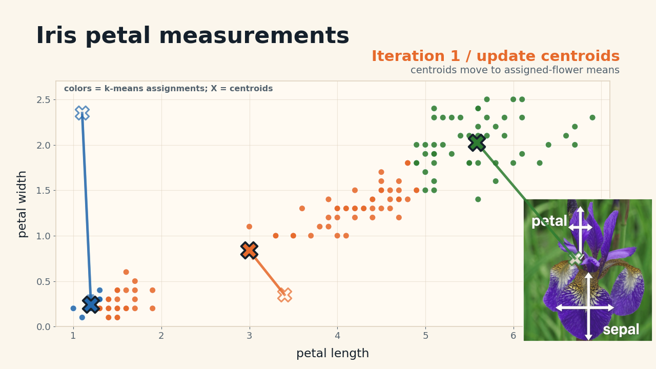
We use the famous iris dataset to demonstrate the k-means algorithm. Each point in the scatter plot represents a flower, where x and y are two measurements of the flower. We want to cluster these points into 3 groups, which ideally correspond to the three species of iris in the dataset. The purpose of K-means is to minimize the objective function value, also known as inertia in K-means, which related to the sum of distances from each point to its assigned centroid.
K-means involves several steps:
First, we initialize the centroids, which can be done in various ways, but for this example, we will use a fixed initialization to ensure that our results are reproducible. Then we perform one run of algorithm, which consists of two main steps: the assignment step, where we assign each data point to the nearest centroid, and the update step, where we recompute the centroids as the mean of the assigned points. We can see the color of points change as they get reassigned to different clusters, and the centroids move as they get updated.
We repeat these steps until convergence, which typically happens when the assignments no longer change. The key point here is that each update depends on the previous state of the centroids and assignments, creating a sequential dependency that can be a bottleneck in terms of performance.
Why k-means works here
K-means is a useful test.
Exposes broad iterative pressures.
Assignment-update shape.
assign
Nearest centroid.
→
update
Recompute centroids.
→
repeat
Stop when stable.
Repeated distance work.
N × K × d
samples × clusters × dimensions.
↻
Sequential state visibility.
Validation contract.
Same data.
Harder scenarios.
Overlap.
Bottleneck shapes.
Loops.
Why it generalizes.
Broad iterative pressure.
Pressure: N × K × d per iteration.
K-means is a useful test case for our framework because it exposes broad iterative pressures that are common in many statistical algorithms. The assignment-update shape of K-means creates a bottleneck due to the repeated distance calculations, which have a computational complexity of N × K × d, where N is the number of samples, K is the number of clusters, and d is the data dimensions.
We can validate our implementation by ensuring that we are using the same data, the same initialization, the same stopping criteria, and the same objective function. We can also test our implementation under harder scenarios, such as when there is overlap between clusters, when there is imbalance in cluster sizes, when there are outliers, or when we are working in high-dimensional spaces. By identifying the bottleneck shapes in our code, such as loops, algebraic operations, or array manipulations, we can apply the appropriate optimization techniques. The iterative nature of K-means means that these pressures are repeated across iterations, making it a good example to demonstrate our framework for validating and optimizing statistical code.
Simulation result before speed result
Did k-means recover groups?
Simulation provides the truth.
ARI recovery score.
1 = perfect. 0 ≈ random baseline.
Can be negative for worse-than-chance agreement.
Scenario stressors.
Separation. Dimension. Outliers. Imbalance.
Before timing.
Speed fails without recovery.
Scenario difficulty summary.
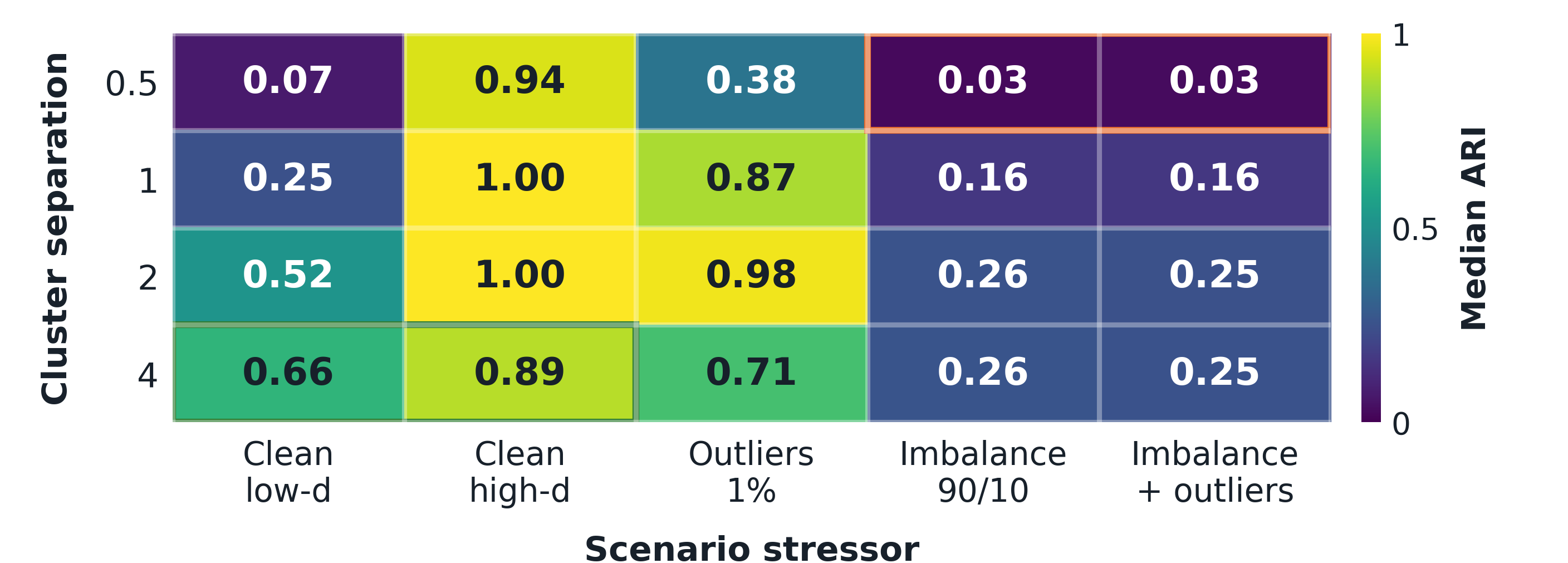
Before optimizing, we must ask: did K-means really recover the true clusters? Therefore, we need to validate the method first.
In our simulations, we use the Adjusted Rand Index (ARI) as a recovery score, where 1 indicates perfect recovery and 0 indicates a random baseline. We test our implementation under various scenario stressors, such as separation between clusters which related to the overlap of clusters, dimensionality of the data, presence of outliers, and imbalance in cluster sizes. The key point is that we should not accelerate our code until we are satisfied with its performance. In the process of algorithm development, we usually detect what we called "failure modes" where the method does not perform well. In this plot, we find that the method performs poorly under certain scenarios.
Although we can optimize our algorithm's performance with statistics, to simplify this presentation, we just skip that steps and assume its ready for optimization. We will directly move on to the validation checks that we use to ensure that our optimized code produces the same results as our reference implementation.
Reference gate
Compare against reference.
Time only after matching.
Same data.
Same initialization.
Same stop.
↓
Readable reference. Executable oracle.
↓
Numba. NumPy. JAX. Must preserve results.
↓
Compare inertia + labels. Stay below tolerance.
main check
3.1e-14
Max inertia diff.
Label agreement: ARI vs reference = 1.0.
tolerance
1e-8
Skip memory-risk rows explicitly.
As previously mentioned, we use same data, same initialization, same stopping criteria, and same objective function to validate our implementation. We already have a reference implementation in NumPy that serves as our executable oracle. When we implement our optimized versions using Numba, JAX, or other tools, we need to ensure that they preserve the results of the reference numpy implementation. To compare the results, we look at both the objective function value and the predicted labels.
We set a tolerance level for the difference in objective function, which is 1e-8 (1 times 10 to the minus 8). In our tests, we observed a maximum difference of 3.1e-14 (3.1 times 10 to the minus 14), which is well below our tolerance threshold. Additionally, we check that the label agreement, measured by ARI, is equal to 1.0, indicating perfect agreement between our accelerated implementation and the reference implementation. By passing these checks, we can be confident that our optimized implementations are correct.
Implementation shape
Three ways to compute.
Same validation. Three expressions.
NumPy
Dense matrix algebra.
x2 = sumsq(X)[:, None]
c2 = sumsq(C)[None, :]

dist2 = x2 + c2 - 2 * (X @ C.T)

labels = argmin(dist2, axis=1)
Shape: BLAS-backed algebra.
Numba
Keep explicit loops.
@njit(parallel=True)
for i in prange(n):
    best = inf

    for k in range(K):
        dist = sqdist(X[i], C[k])
        if dist < best:
            best = dist
            labels[i] = k
JAX / GPU
Array expression on device.
@jax.jit
def assign(X, C):
    x2 = sumsq(X)[:, None]
    c2 = sumsq(C)[None, :]

    dist2 = x2 + c2 - 2 * (X @ C.T)
    return jnp.argmin(dist2, axis=1)
Shape: Batch for accelerators.
Match expression to bottleneck shape.
Here are the details of the three implementations for the assignment step of K-means. The first implementation uses NumPy to express the distance calculations as dense matrix algebra. We compute the squared distances using the formula that involves the sum of squares of the data points and centroids, and then we use matrix multiplication to compute the cross term. This approach can be efficiently executed using BLAS libraries, which are optimized for performance on CPUs. The second implementation uses Numba to write loops that compute the distances and find the nearest centroid for each data point. This approach allows us to parallelize the computation across CPU cores, which can be beneficial for smaller datasets or when the distance calculations are not easily expressed as matrix operations. The third implementation uses JAX to write a similar expression to the NumPy version, but it is compiled to run on a GPU for potentially faster execution. JAX allows us to write code that looks like NumPy, but it can be executed on different hardware backends, including GPUs and TPUs. Each of these implementations has its own advantages and trade-offs depending on the specific bottleneck shape.
Scale tier
Engine depends on shape.
Read shapes, not rankings.
Scalar-heavy loops.
N=100k, d=10, K=5
Numba fits loop-heavy work.
Dense distance algebra.
N=1M, d=256, K=50
NumPy fits dense algebra.
Massive regular batches.
large, regular array work
JAX GPU fits large regular batches.
Shape determines the tool.
So, which engine is the best choice? It depends on your bottleneck's shape.
In the first row, K and d are small. The work is scalar-loop heavy: many simple point-to-centroid comparisons. Here Numba is a natural fit because we can keep the algorithm close to explicit loops, remove Python interpreter overhead, and avoid building a large dense distance matrix.
In the second row, the shape changes. With larger dimension and more clusters, the distance computation becomes dense algebra. The BLAS libraries that back NumPy are highly optimized for this kind of work. That is why NumPy can beat numba here.
In the third row, the work is large, regular, and batched enough for the accelerator path. JAX on GPU can help, but only because there is enough device-friendly work to transfer data, batching, and pipeline overhead. It is not a free GPU win.
So the conclusion is not “Numba is best,” “NumPy is best,” or “GPU is best.”
The conclusion is: validate the result first, identify the bottleneck shape, then choose the suitable tool that fits that shape.
Workload 2
Permutations. Resampling inference pressure.
Expensive with many features.
Then, comes the permutation test.
Method visualization
Permutation test scaling.
Shuffle labels. Build null.
One resampling loop.
Shuffle labels.
Compute group differences.
Repeat for null.
Independent repeats create work.
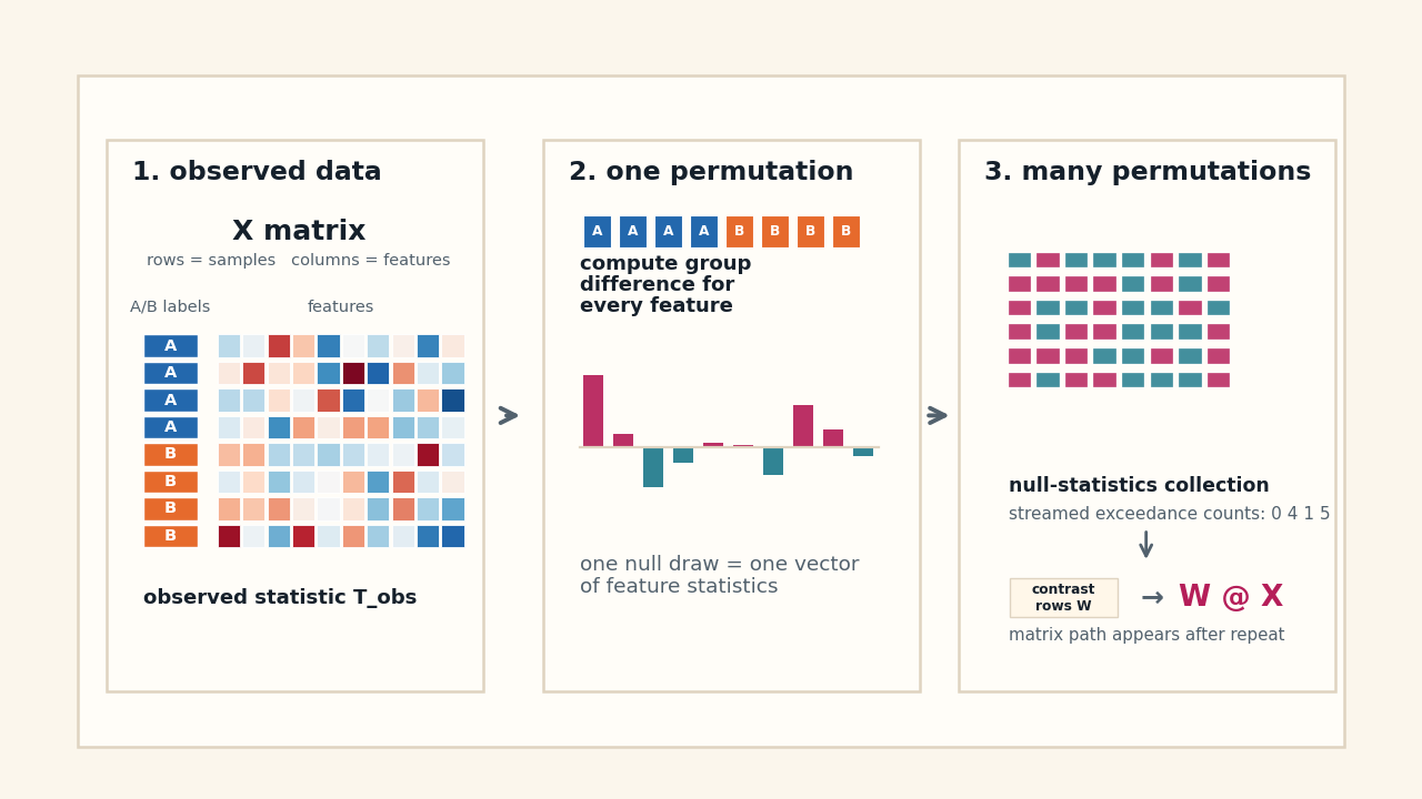
In permutation tests, we repeatedly shuffle the labels of our data and compute the group differences to build a null distribution. This process involves three main steps. Here's our data. Each row is a sample, and each column is a feature. We have two groups A and B, and we want to test if there are significant differences between these groups for each feature.
First, we shuffle the labels while keeping the data matrix X unchanged. Second, we compute the group differences for each feature, which gives us a statistic for every feature. Third, we repeat this process many times to build the null distribution. The repeats are independent, but they are not free in terms of computational cost. With R permutations and p features, the amount of work scales as R times p, which can become a performance problem when there are many features or many permutations. The W @ X notation on the figure represents the later implementation view, where we can batch the permutation using matrix operations. But, the underlying statistical question remains the same.
Code shape
Same math. New shape.
Rewrite the repetition.
Reference loop.
for r in range(R):
    labels_r = same_permutation_stream[r]
    stat[r, :] = group_difference(X, labels_r)
Optimized path.
for W_batch in contrast_batches(
        same_permutation_stream):
    T = W_batch @ X
    counts += abs(T) >= abs(T_obs)
W_batch: batch_R × n
X: n × p
T: batch_R × p
Stream avoids R × p matrix.
The reference loop implementation of the permutation test iterates over each of the R permutations, computes the group difference statistic for each feature, and stores it in an R by p matrix. This approach is straightforward but can be inefficient due to the large size of the resulting matrix. In contrast, the optimized path rewrites the computation to avoid explicitly forming the R by p matrix. Instead, it processes batches of permutations using a contrast matrix W_batch that encodes the shuffled labels. By multiplying W_batch with the data matrix X, we can compute the statistics for a batch of permutations at once. This streaming approach allows us to handle larger workloads more efficiently while still producing the same mathematical results.
Correctness gate 1
Equivalence: loop vs. matrix.
Verify before timing.
Same inputs.
Same data.
Reference.
Loop formulation.
Optimized path.
Matrix formulation.
validation grid
18 × 5
workloads × seeds
0.0
max |p diff|
9.4e-16
max |stat diff|
1e-6
validation tolerance
Acceptance criteria
✓
P-values agree exactly.
✓
Stat differences are roundoff dust.
✓
Optimized path approved.
Same result. Faster code.
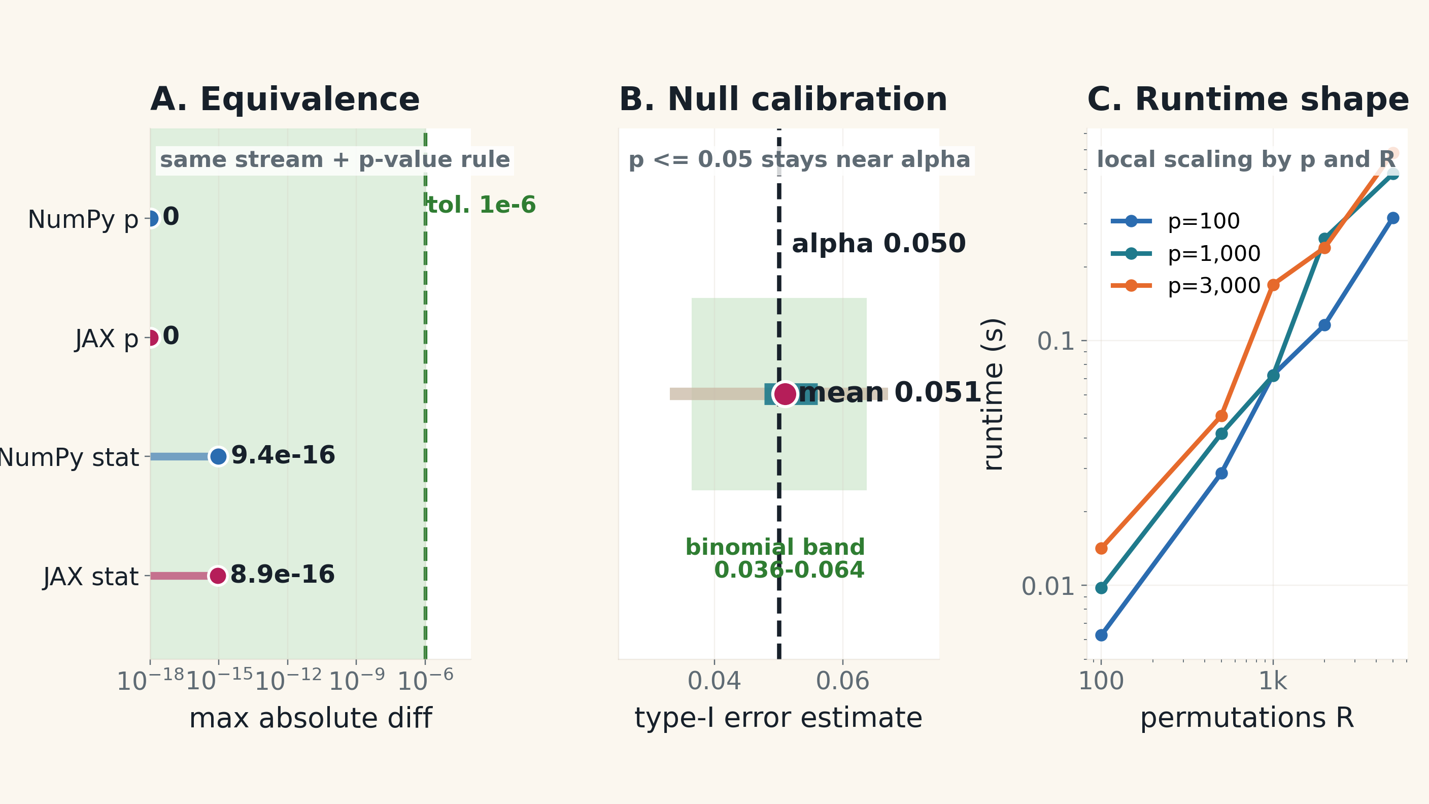
Before we can trust the optimized path, we need to verify that it produces the same results as the reference loop implementation. We run both implementations on the same inputs, which means using the same data matrix X and the same stream of shuffled labels. The reference implementation computes the statistics one by one in a loop, while the optimized path computes them in batches using matrix operations. We compare the outputs of both implementations across a several validation grid and random seeds. The acceptance criteria including the maximum absolute difference in p-values and statistics which are all below our tolerance threshold.
CORRECTNESS GATE 2
Null calibration check.
Type-I error near 0.05.
Why calibrate? Checks inference behavior.
Observed check. Error estimate ≈ 0.051.
Before scaling. Acceptable for scaling.
calibrated
0.051 Type-I error estimate.
Calibration ruler
feature-level binomial band 0.036-0.064
0.025 0.035 0.045 0.055 0.065 0.075
Dashed: Nominal alpha 0.050.Dot: Observed mean 0.051.
Band is per-feature binomial variation, not CI for the mean.
Calibration checks inference.
Equivalence: code. Calibration: inference.
We also check the calibration of our permutation test under the null hypothesis. Here we generate data where there is no true effect (the null condition) and run our permutation test to see how often it produces false positives. The Type-I error rate is the proportion of times we incorrectly reject the null hypothesis when it is actually true. We want this rate to be close to our nominal alpha level of 0.05. In our calibration check, we estimate the Type-I error rate and find it to be approximately 0.051 which we consider to be well-calibrated.
LOCAL SCALE SIGNAL
When does runtime bend?
p and R reveal bottlenecks.
Same statistic.
Same stream and definition.
equivalence passed
Local runtime.
MacBook. Batched NumPy. n=500.
warm median
Scale question.
When does runtime explode?
local runtime scaling
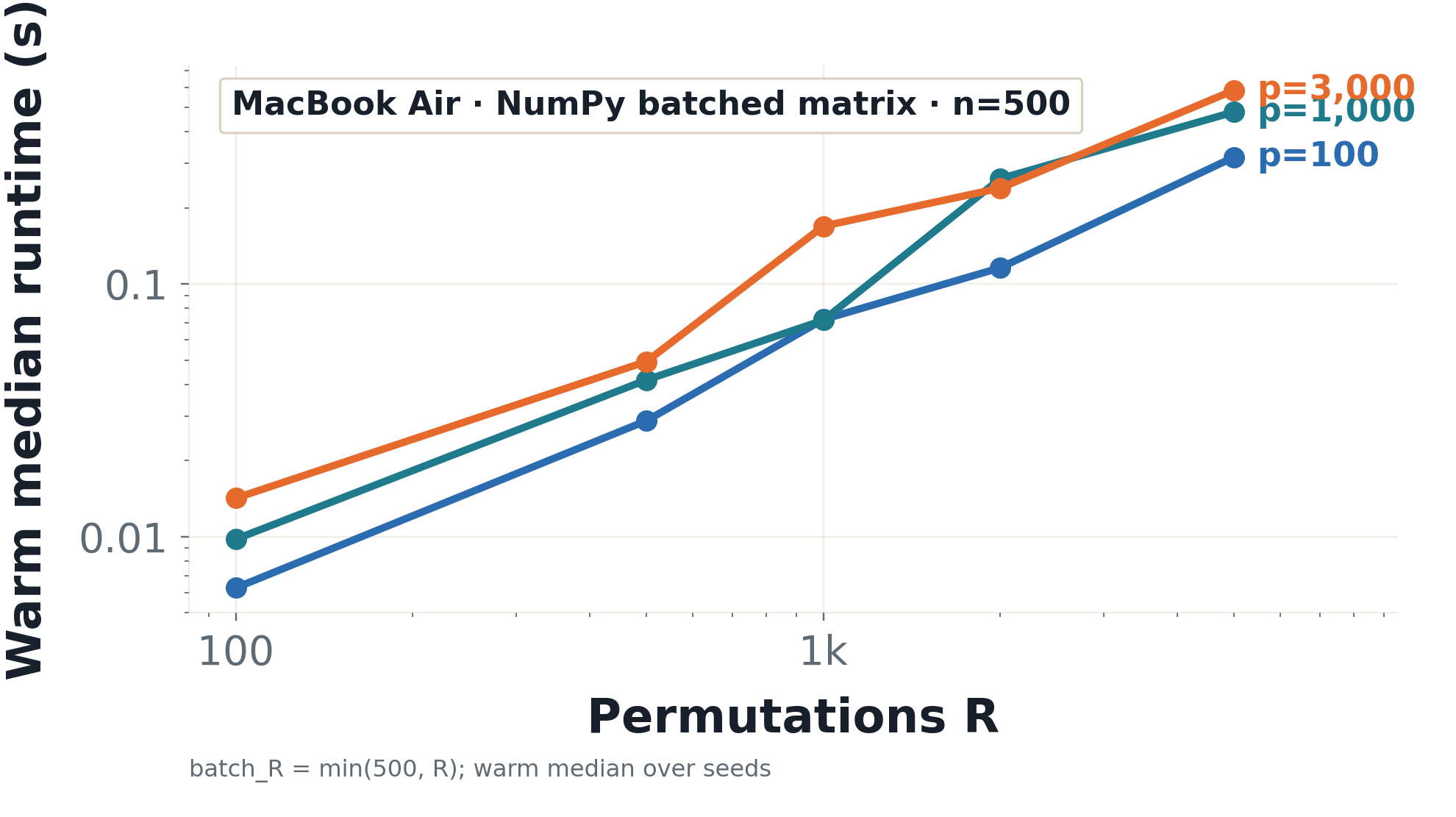
MacBook Air local tier · NumPy batched matrix · n=500 · warm median. Shape signal. Not leaderboard.
Local runtime motivates server/GPU.
Before we can optimize for performance, we need to understand how the runtime of our permutation test scales with the number of features p and the number of permutations R. We run a local runtime scaling experiment on a MacBook Air using a batched NumPy implementation with n=500 samples. The resulting figure shows how the runtime changes as we vary p and R. This local runtime signal helps us identify when the runtime starts to explode, which can inform our decisions about when to move to more powerful hardware like servers or GPUs. By analyzing this scaling behavior, we can better understand the computational bottlenecks in our implementation and make informed choices about optimization strategies.
DECISION MAP
When do GPUs help?
Requires massive R × p.
Scope Speedup: CPU vs. GPU e2e.
Explicit OOM cells. Unavailable for GPUs.
Validation and batching unlock GPUs.
Transfer included; compile excluded. Not a leaderboard.
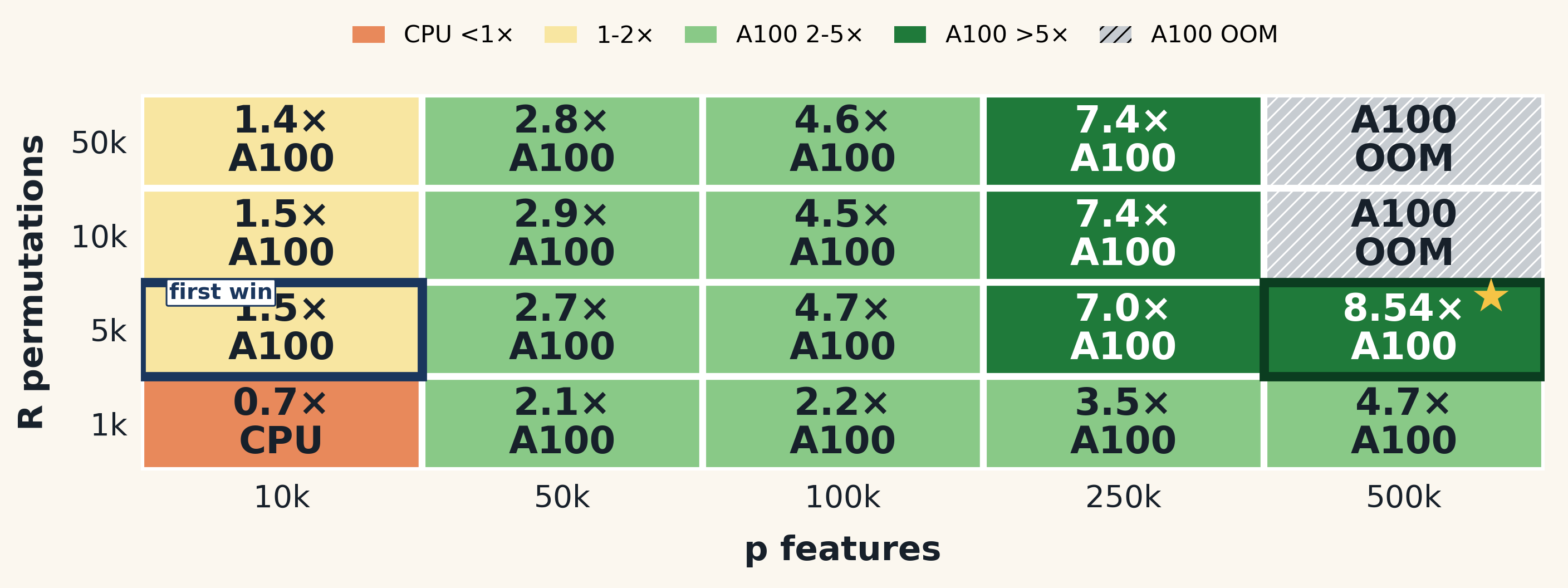
To determine when GPUs can provide a speedup for our permutation test, we create a map that compares the end-to-end runtime of CPU and GPU implementations in a Linux server across different values of p (number of features) and R (number of permutations). Here, we find that GPUs can offer significant speedups when the workload is sufficiently large, for example, R=5k and p=500k, GPU can have a 8.5x speedup.
However, we also note that when the workload is large enough to cause out-of-memory (OOM) errors on the GPU, the CPU of our server still works, which can be considered a win for the CPU in those cases. The decision map helps us understand the conditions under which GPUs can be beneficial and when we might need to rely on CPU resources instead.
PARALLELISM
Parallelism helps. Then flattens.
Measure time and marginal gain.
Total time drops.
Parallelism helped early.
runtime
Returns flatten.
Gains shrink later.
marginal gain
Memory matters.
Workers consume memory.
memory
Capture early speedup.
Execution model matters next.
Parallelism helps — but only up to a point.
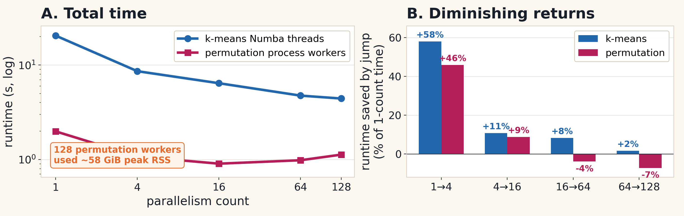
On the left, you can see the good news first. When we move from one worker to a few workers, total runtime drops a lot. That is the speedup we want to capture.
But the right panel tells the second half of the story. Each jump gives us a smaller marginal gain. The first jump is
very valuable; later jumps are much less valuable. And for the permutation workload, adding more workers at the high end can even make things worse.
So the lesson is not simply “add more workers.”
The practical rule is: use parallelism to capture the early speedup, then watch the marginal gain. When the curve
flattens, more workers are no longer free.
EXECUTION MODEL
No-GIL changes the process-vs-thread tradeoff.
CPU-bound Python permutation/resampling work over shared in-memory data.
Standard GIL builds
~1.02×
1 → 16 workers
py314 stays flat
CPython 3.14t / free-threaded
4.77×
1 → 16 workers
threads scale this workload
Execution-model payoff
2.43× faster
32% less peak RSS
ThreadPool vs ProcessPool
The claim is not that Python is automatically faster; it is that free-threaded CPython makes threads a plausible shared-data parallel strategy for this workload shape.
Before choosing Numba, NumPy, or JAX, we can also choose how the work is executed: processes, threads, or accelerator kernels.
The workload here is permutation-style resampling: many mostly independent Python tasks running over data that we would like to keep shared in memory.
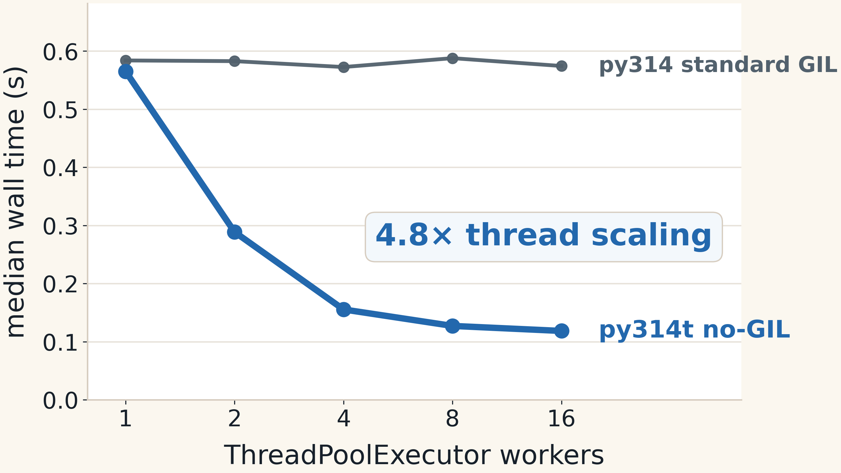
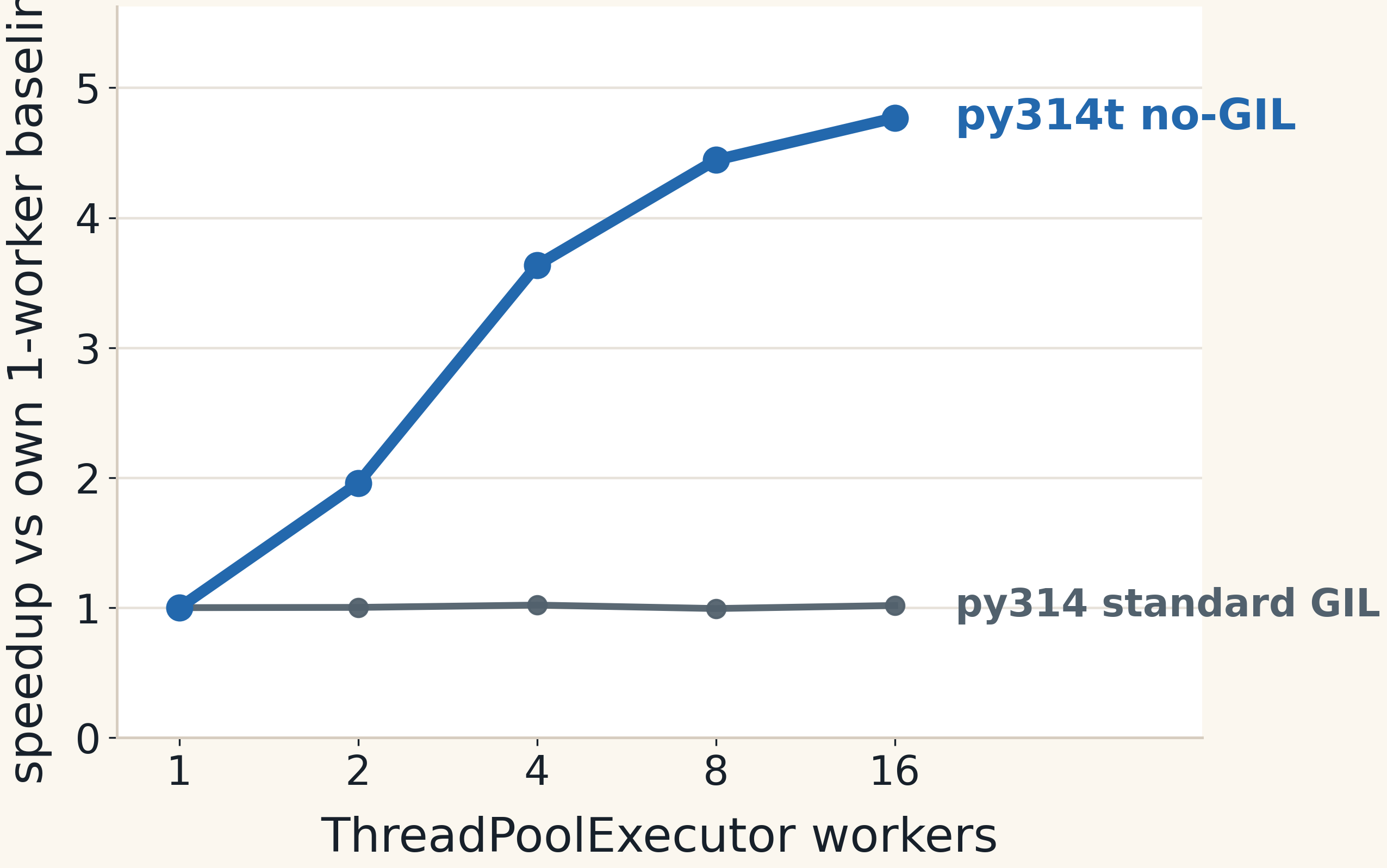
With the standard GIL build, adding ThreadPoolExecutor workers does not give meaningful CPU parallelism. From 1 to 16
workers, the runtime is essentially flat, no improvement.
With the free-threaded CPython build, the same thread-based design scales to about 4.77× from 1 to 16 workers. That is
the important evidence: the difference is not Python version, it is whether Python threads can execute this
CPU-bound work in parallel.
This does not mean every Python program gets faster. It works here because the workload has the right shape: mostly
independent CPU-bound Python work, shared read-heavy data, and limited cross-thread coordination.
That is why the payoff is not only runtime. In the pool comparison, the ThreadPool path is about 2.43× faster than the
ProcessPool path and uses about 32% less peak RSS, because it can keep the large in-memory data inside one process
instead of paying process, serialization, IPC, and memory overhead.
So the takeaway is: free-threaded CPython changes the process-versus-thread tradeoff for this workload shape. Threads
become a real option when memory sharing matters, the work is independent enough, and the statistical validation still
passes.
Connecting the tools
What each tool solved.
Match tool to shape.
Numba
Bottleneck:
Solved: K-means assignment.
NumPy / BLAS
Bottleneck:
Solved: Distance identity.
Threads / workers
Bottleneck:
Solved: Permutation workers.
JAX / GPU
Bottleneck:
Solved: Streamed W @ X.
Same statistic. Different tool.
To summarize: Numba conquered CPU loops. NumPy conquered dense algebra. JAX provided GPU acceleration. And Free-threaded Python resolved shared-memory scaling limits.
DECISION GUIDE
Evidence to tool.
Follow bottlenecks, not the leaderboard.
1 Simulate
→
2 Validate
→
3 Find the bottleneck
→
4 Pick the suitable tool
Hot loop
Signal Loop dominates.
Limit Python overhead.
Move Numba.
k-means loops
Matrix algebra
Signal Matrix operations.
Limit Dense kernel.
Move NumPy / BLAS.
distance identity
Repeat work
Signal Repeats over data.
Limit Scheduling / memory.
Move Threads or workers.
permutation workers
Large streamed batch
Signal Batches fit device.
Limit Regular array work.
Move JAX / GPU.
GPU batch
Validate first. Move bottlenecks.
This brings us to the final decision guide. The workflow is systematic: simulate, validate, identify the bottleneck, and then choose the suitable tool that preserves the checked result.
On a personal note, I think choosing a computational engine is a lot like choosing transportation. I traveled here to
LA from Hong Kong. For that distance, I took an airplane; nobody expected me to swim across the Pacific. Then,
from LA to Long Beach, I took the Metro. Interestingly, my AI routing app confidently recommended a two-and-a-half-hour bus ride instead. That was a useful reminder: automation can suggest a route, but we still have to understand the constraints. And finally, from my hotel to this venue, I walked about 5 min. For that short local trip, walking had almost zero overhead. Calling a car would not have made it better.
Computational bottlenecks work the same way. You do not choose the vehicle first; you look at the shape of the trip. If the bottleneck is a tight local numerical loop—many small point-to-centroid comparisons—Numba is the right vehicle. It keeps the algorithm explicit but removes Python loop overhead. If the bottleneck becomes dense matrix algebra, NumPy is the express train, utilizing optimized linear algebra underneath. If the bottleneck is repeated CPU work over shared arrays, then threads or Python 3.14 can help. And if the workload is massive, regular, and batched enough to amortize transfer overhead, that is when JAX on an A100 becomes the long-haul flight.
So the rule is not: always use Numba, always use NumPy, or always use a GPU. The rule is: validate first, understand the shape of the journey, then move the bottleneck with the suitable tool that fits.
AI coding tools
AI scales the workflow. We own the claims.
AI automation.
Implementation variants.
Scenario runners.
Metadata capture.
Plot regeneration.
Result manifests.
Scientific judgment.
Statistical target.
Data assumptions.
Validation criteria.
Hard-case interpretation.
Scientific claims.
AI automates. Humans claim.
I believe everyone here have tried AI coding tools. They are impressively good at automating many of the mechanical tasks involved in coding and experimentation. Prevously, there's a page for the effort for translating the original NumPy loop into a Numba version or jax version. With AI coding tools, such translation can be done without much manual effort. Even if you want to rewrite every code in Rust, AI can help you with that too.
However, as researchers, we need to take ownership of these scientific decisions and claims. AI can be a powerful assistant in automating tasks, but it is ultimately up to us to ensure that our work is scientifically valid and that we are making accurate claims based on our findings.
Close
Make the statistic testable.
Clear enough to validate. Fast enough to scale.
To summarize the key message of this presentation: when optimizing a statistical method, we should first focus on making the statistic testable. This means ensuring that we have a clear and correct implementation that can be validated against a reference implementation. Once we have established correctness and understand the behavior of our implementation, we can then identify the bottlenecks in our code and apply targeted optimizations to make it fast enough to scale to larger datasets or more complex analyses. The principle is to prioritize correctness and testability before performance, as a fast implementation that produces incorrect results is not useful. By following this approach, we can ensure that our optimized code is both scientifically valid and efficient.
Thank you
Questions?
Slides. Reproducible artifacts.
github.com/LucaJiang/FastStatisticalModels4Python
Slides. Reproducible artifacts.
Thank you for your attention. If you have any questions, please feel free to ask. The slides and reproducible artifacts for this presentation are available on GitHub at the following this link. You can also scan the QR code on the right to access the repository directly.
Backup: Evidence scope.
Evidence map. Different questions.
Why three environments?
MacBook = validation. Equivalence. Calibration. Local shape.
Server = scale. Parallelism. Shape scaling. Memory sweeps.
GPU = accelerator pipeline. Break-even evidence. Streamed reduction.
Detailed metrics in repository.
If you are wondering why we didn't just build one massive hardware leaderboard, the answer is scope. Each environment answers a different question. The MacBook establishes local validation. It gives us local shape signals. The server CPU answers scaling and parallelism questions. The GPU only enters the picture to ask: does this validated, streamed pipeline actually win? It is an evidence map, not a leaderboard.
Backup: Local validation.
Validation inventory.
Code. Inference. Runtime shape.
If you want to see the full local permutation checks, here is the inventory. It combines main-path equivalence, null calibration, and the local runtime shapes. This is all local MacBook evidence. We run all of this before we ever touch a server or a GPU.
Backup: K-means loops.
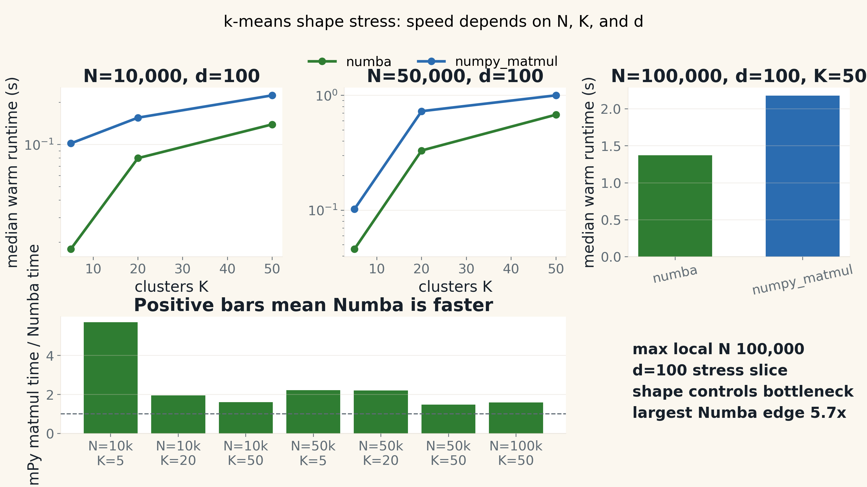
Numba wins loop shapes.
Loops favor Numba. Algebra favors BLAS.
Someone usually asks why Numba looks so fast locally but loses on the server. Look at the shape. This is local MacBook shape-stress evidence. Over a thousand rows. All passing. Numba dominates when the shape is pure explicit loop work. But when you move to a server and the shape widens into dense distance algebra, BLAS takes over. And at massive device-friendly scale, the GPU wins. It never contradicts. It just changes shape.
Backup: Statistical power.
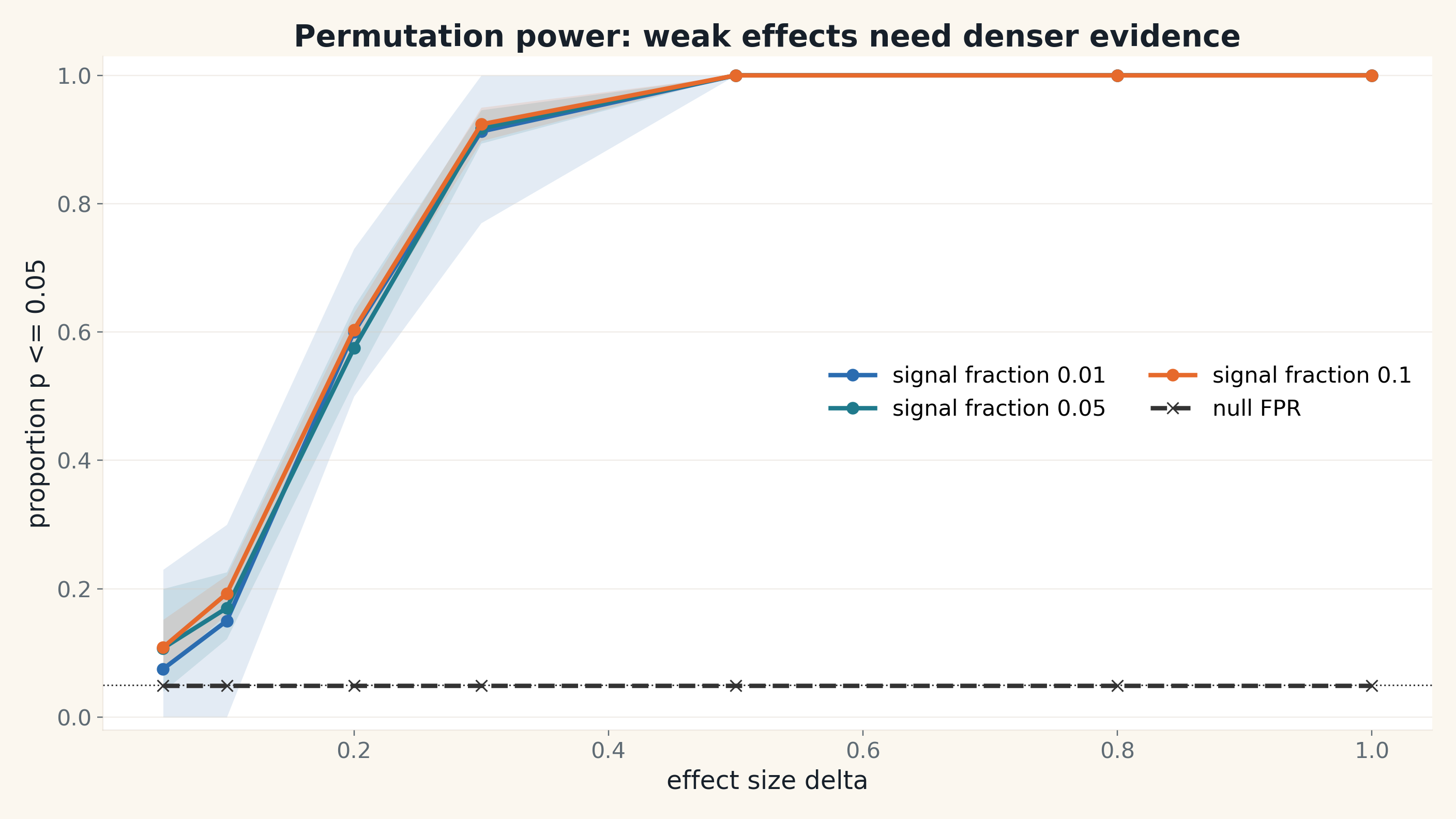
Power vs. effect size.
Do we detect strong signals?
Strong signals yield high power.
If you want statistical validation beyond just the null calibration, here is the simulated power curve. This is not a speed result. It is pure statistics. The reading is very simple. Weak effects have low power. Stronger simulated signals are easier to detect. The inference behaves exactly as it should.
Backup: batch_R=8192.
BACKUP: GPU TUNING
Backup: what batch_R tuning showed
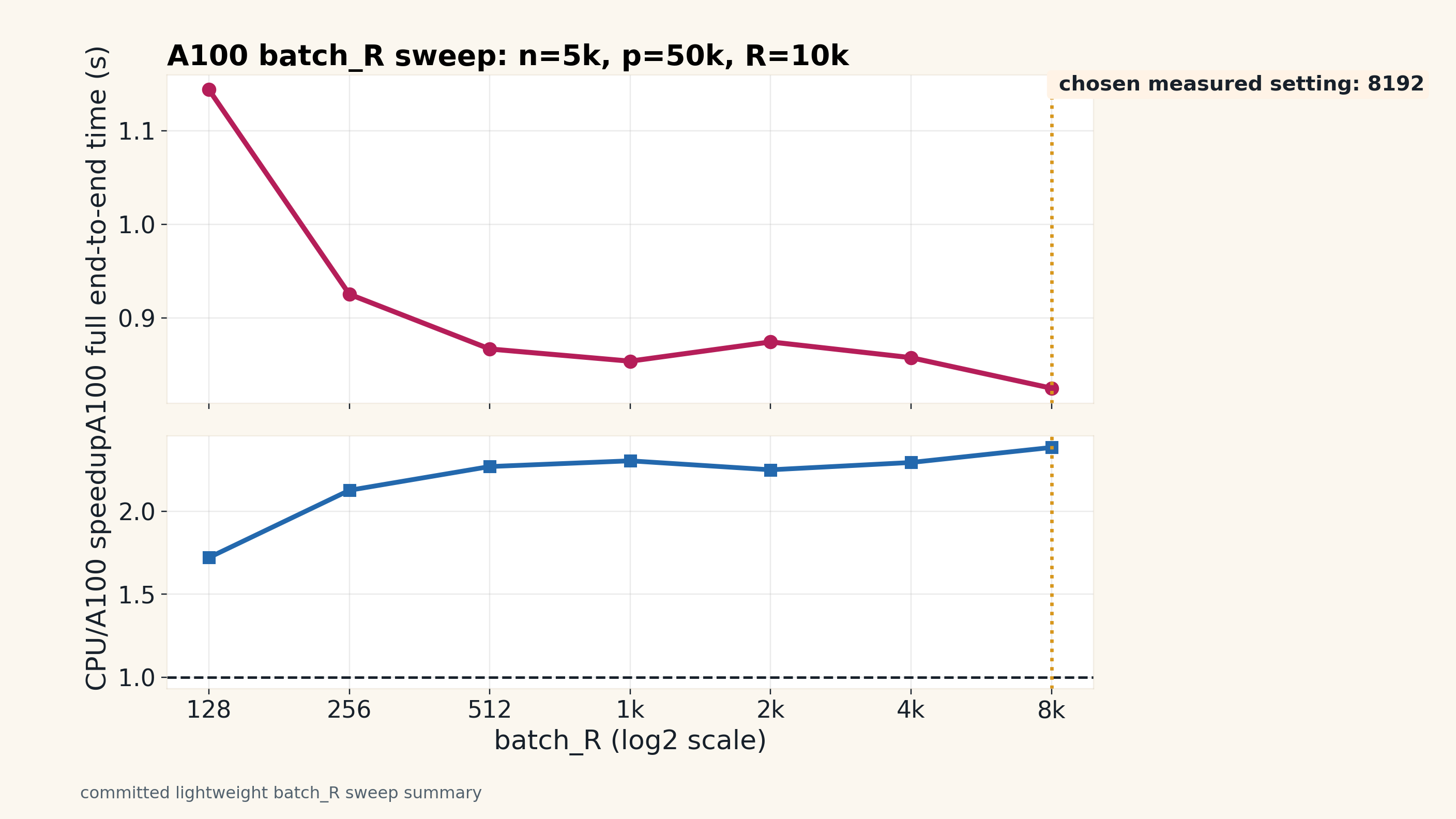
Larger batches amortized overhead; 8192 was fastest only within this measured grid.
Timing improved most at small batch_R; after 512-1024 the curve mostly flattened. 8192 is the fastest accepted value measured here.
Definition
batch_R = permutation rows processed in one A100 batch.
Trend
Small batches were slower; larger batches reduced stream overhead.
Diminishing returns
Most of the gain appeared by 512-1024; later points were nearly flat.
Claim boundary
8192 was fastest in this measured grid. Larger values were not tested here.
batch_R tunes pipeline overhead; it does not change the statistical question.
This backup slide is about the trend, not a proof of optimality. batch_R is the number of permutation rows processed in one A100 batch. In this committed sweep, small batches were slower because the streamed path paid more scheduling and loop overhead. Increasing batch_R reduced that overhead, but the gains flattened after roughly 512-1024 and the curve is not perfectly monotone. 8192 was the fastest accepted value in the measured 128-8192 grid, so it was used as the chosen setting for the later A100 decision map. Larger batch_R values were not part of this committed sweep; they could be faster, slower, or fail because of memory or autotuning. batch_R changes scheduling, not the permutation statistic or p-value definition. Full end-to-end timing remains the criterion: compile excluded, transfer included, kernel-only excluded.
Backup: AI workflow.
What the agent automated.
Experiment orchestration. Runners. Scenarios. Manifests.
Visualization surface. Regenerated figures from CSVs.
Repository surface. Commands. Summaries. QA notes.
AI automated. Humans claimed.
For those curious about the AI agent workflow, here is what it actually automated. It handled experiment orchestration. It built the resumable runners and scenario grids. It regenerated all the figures from the CSV results. It kept the repository clean with reproducible commands and QA notes. It massively widened our experimental surface area. But again, the statistical claims stayed entirely human-owned.
Backup: standard GIL vs free-threaded
Scaling evidence.
Compare scaling, not base speed.
ThreadPoolExecutor workers
Build
1 worker
16 workers
Ratio
py314 standard GIL
0.584s
0.574s
1.02×
CPython 3.14t free-threaded
0.565s
0.119s
4.77×
CPython 3.14 answers
the standard-GIL baseline; CPython 3.14t answers the free-threaded execution-model question.
ThreadPool vs ProcessPool runtime
py314 ProcessPool 0.571s
3.14t ThreadPool 0.235s
2.43× faster
ThreadPool vs ProcessPool peak RSS
py314 ProcessPool 1.017 GiB
3.14t ThreadPool 0.692 GiB
32% lower
ThreadPool shares dataset.
The py313 control is not present in the local benchmark outputs, so this backup uses only the
available py314 and py314t data. The chart normalizes each interpreter to its own one-worker baseline. The standard
GIL build stays flat. The free-threaded build scales on this CPU-bound Python workload. The pool rows show why the
execution model matters: ProcessPoolExecutor can work around the GIL, but threads avoid the memory and serialization
costs for shared data.