Expectation-Maximization (EM) algorithm for Linear Mixed-Effect Model (LMM)

• Expectation-Maximization (EM) algorithm for Linear Mixed-Effect Model (LMM)
  • Model Description
  • Statistical Inference in LMM
    • Complete Data Log-Likelihood
    • Statistical Inference in E-Step
    • Statistical Inference in M-Step
    • Statistical Inference in Incomplete Data Log-Likelihood
  • The EM Algorithm: n >= p
    • E-step
    • M-step
    • Incomplete Data Log-Likelihood
    • Pseudocode
  • The EM Algorithm: n < p
    • Woodbury Matrix Identity
    • Eigenvalue decomposition
    • Pseudocode
  • Codes and Results
    • Codes
    • Results
  • TODO:

Model Description

The relation between OLM and LMM can be found in The Introduction of Linear Mixed-Effect Model.

The linear mixed-effect model (LMM) is a statistical model that accounts for both fixed effects and random effects in a linear regression model. It is used for modeling data where observations are not independent or identically distributed.

Consider a dataset $\{\mathbf{y}, \mathbf{X},\mathbf{Z}\}$ with $n$ samples, where $\mathbf{y} \in \mathbb{R}^n$ is the vector of response variable, $\mathbf{X} \in \mathbb{R}^{n \times p}$ is the matrix of $p$ independent variables, and $\mathbf{Z} \in \mathbb{R}^{n \times c}$ is another matrix of $c$ variables. The linear mixed model builds upon a linear relationship from $\mathbf{y}$ to $\mathbf{X}$ and $\mathbf{Z}$ by
$$\begin{equation} \mathbf{y} = \underbrace{\mathbf{Z}\mathbf{\omega}}_{\text {fixed}} + \underbrace{\mathbf{X}\mathbf{\beta}}_{\text {random}} + \underbrace{\mathbf{e}}_{\text {error}}, \end{equation}$$
where $\mathbf{\omega} \in \mathbb{R}^c$ is the vector of fixed effects, $\mathbf{\beta} \in \mathbb{R}^p$ is the vector of random effects with $\mathbf{\beta} \sim \mathcal{N}(\mathbf{0}, \sigma^2_\mathbf{\beta} \mathbf{I}_p)$, and $\mathbf{e} \sim \mathcal{N}(\mathbf{0}, \sigma^2_e \mathbf{I}_n)$ is the independent noise term.

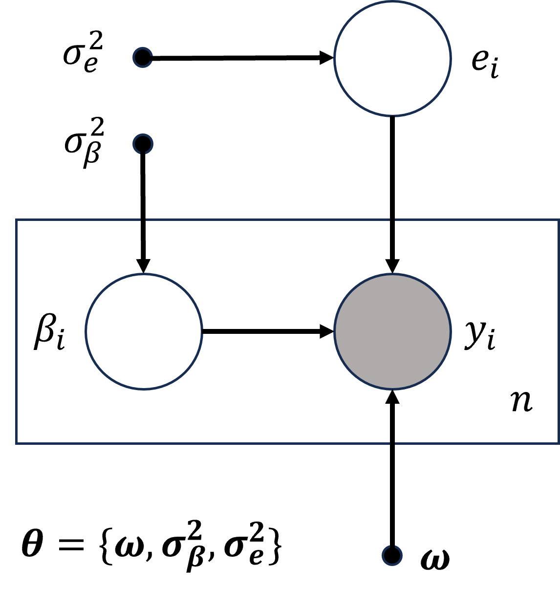
Let $\mathbf{\Theta}$ denote the set of unknown parameters $\mathbf{\Theta} = \{\mathbf{\omega}, \sigma^2_\mathbf{\beta}, \sigma^2_e\}$. Under the framework of EM algorithm, we can treat $\mathbf{\beta}$ as a latent variable. Below is the directed acyclic graph below for our model.

The EM algorithm is an iterative algorithm that alternates between the E-step and the M-step until convergence. In the following sections, we will first find the posterior distribution of $\mathbf{\beta}$ given $\mathbf{y}$ and $\hat{\mathbf{\Theta}}$ in the E-step and calculate the $Q$ function. Then we will find the ML estimator of $\mathbf{\Theta}$ which is used in M-step. Finally, we will calculate and track the marginal data log-likelihood $\ell(\mathbf{\Theta})$ to check the convergence of the algorithm.

Statistical Inference in LMM

Complete Data Log-Likelihood

The complete data log-likelihood is given by
$$\begin{equation} \begin{split} \ell(\mathbf{\Theta}, \mathbf{\beta}) &= \log p(\mathbf{y}, \mathbf{\beta}| \mathbf{\Theta})\\ &= \log p(\mathbf{y}| \mathbf{\beta}, \mathbf{\Theta}) + \log p(\mathbf{\beta}| \mathbf{\Theta})\\ &= -\frac{n}{2} \log (2\pi) -\frac{n}{2} \log \sigma_e^2 - \frac{1}{2\sigma_e^2} \|\mathbf{y} - \mathbf{Z}\mathbf{\omega} - \mathbf{X}\mathbf{\beta}\|^2\\ &\quad -\frac{p}{2} \log (2\pi) -\frac{p}{2} \log \sigma_\beta^2 - \frac{1}{2\sigma_\beta^2} \mathbf{\beta}^T \mathbf{\beta} \end{split}\end{equation}$$

Statistical Inference in E-Step

The E-step is to compute the expectation of the complete data log-likelihood with respect to the conditional distribution of $\mathbf{\beta}$ given $\mathbf{y}$ and $\mathbf{\Theta}$:
$$\begin{equation} Q(\mathbf{\Theta}|\mathbf{\Theta}^{\text{old}}) = \mathbb{E}_{\mathbf{\beta}|\mathbf{y}, \mathbf{\Theta}^{\text{old}}} \ell(\mathbf{\Theta}, \mathbf{\beta}) \end{equation}$$

Therefore, we need to find the posterior distribution of $\mathbf{\beta}$ given $\mathbf{y}$ and $\mathbf{\Theta}$. However the posterior distribution of $\mathbf{\beta}$ can not be obtained directly. Instead, by applying Bayes' rule, we have
$$\begin{equation} \begin{split} p(\mathbf{\beta}| \mathbf{y}, \mathbf{\Theta}) &= \frac{p(\mathbf{y}| \mathbf{\beta}, \mathbf{\Theta}) p(\mathbf{\beta}| \mathbf{\Theta})}{p(\mathbf{y}| \mathbf{\Theta})}\\ &\propto p(\mathbf{y}| \mathbf{\beta}, \mathbf{\Theta}) p(\mathbf{\beta}| \mathbf{\Theta})\\ &\propto \exp \left\{-\frac{1}{2}(\mathbf{y} - \mathbf{Z}\mathbf{\omega} - \mathbf{X}\mathbf{\beta})^T (\sigma_e^2\mathbf{I}_n)^{-1} (\mathbf{y} - \mathbf{Z}\mathbf{\omega} - \mathbf{X}\mathbf{\beta}) \right\} \\ &\quad \times \exp \left\{-\frac{1}{2} \mathbf{\beta}^T (\sigma_\beta^2 \mathbf{I}_p)^{-1} \mathbf{\beta} \right\} \\ &\propto \exp \left\{-\frac{1}{2}\left( \mathbf{\beta} - \mathbf{\mu}\right)^T \mathbf{\Gamma}^{-1} \left( \mathbf{\beta} - \mathbf{\mu}\right) \right\} \end{split}\end{equation}$$

where $\mathbf{\Gamma} = \left(\frac{\mathbf{X}^T \mathbf{X}}{\sigma_e^2} + \frac{\mathbf{I}_p}{\sigma_\beta^2} \right)^{-1}$ and $\mathbf{\mu} = \mathbf{\Gamma} \mathbf{X}^T (\mathbf{y}-\mathbf{Z}\mathbf{\omega})/\sigma_e^2$. And, the posterior distribution of $\mathbf{\beta}$ is $\mathbf{\beta}|\mathbf{y}, \mathbf{\Theta} \sim \mathcal{N}(\mathbf{\mu}, \mathbf{\Gamma})$. ^[1]

Thus, we have
$$\begin{equation} \begin{split} Q(\Theta|\Theta^{\text{old}}) &= \mathbb{E}_{\mathbf{\beta}|\mathbf{y}, \Theta^{\text{old}}} \left[ \log p(\mathbf{y}, \mathbf{\beta}|\Theta) \right]\\ &= \mathbb{E}_{\mathbf{\beta}|\mathbf{y}, \Theta^{\text{old}}} \left[ \log p(\mathbf{y}| \mathbf{\beta}, \mathbf{\Theta}) + \log p(\mathbf{\beta}| \Theta) \right]\\ &= \mathbb{E}_{\mathbf{\beta}|\mathbf{y}, \Theta^{\text{old}}} \left[ -\frac{n}{2} \log (2\pi) -\frac{n}{2} \log \sigma_e^2 - \frac{1}{2\sigma_e^2} \|\mathbf{y} - \mathbf{Z}\mathbf{\omega} - \mathbf{X}\mathbf{\beta}\|^2 \right.\\ &\quad \left. -\frac{p}{2} \log (2\pi) -\frac{p}{2} \log \sigma_\beta^2 - \frac{1}{2\sigma_\beta^2} \mathbf{\beta}^T \mathbf{\beta} \right]\\ &= -\frac{n+p}{2} \log (2\pi) -\frac{n}{2} \log \sigma_e^{2}-\frac{p}{2} \log \sigma_\beta^2 - \frac{1}{2\sigma_\beta^2} \text{tr}(\mathbf{\Gamma}) - \frac{1}{2\sigma_\beta^2} \mathbf{\mu}^{T} \mathbf{\mu}\\ &\quad - \frac{1}{2\sigma_e^{2}} \left(\|\mathbf{y} - \mathbf{Z}\mathbf{\omega}\|^2 + \text{tr}(\mathbf{X}\mathbf{\Gamma} \mathbf{X}^T) + \mathbf{\mu}^T\mathbf{X}^T \mathbf{X}\mathbf{\mu}- 2(\mathbf{y} - \mathbf{Z}\mathbf{\omega})^T \mathbf{X}\mathbf{\mu} \right) \end{split}\end{equation}$$

Note that $\mathbb{E}[\mathbf{\beta}^T \mathbf{\beta}] = \text{tr}(\mathbb{V}[\mathbf{\beta}]) + \mathbb{E}[\mathbf{\beta}]^T \mathbb{E}[\mathbf{\beta}] = \text{tr}(\mathbf{\Gamma}) + \mathbf{\mu}^T \mathbf{\mu}$ and $\mathbb{E}[(\mathbf{X}\mathbf{\beta})^T (\mathbf{X}\mathbf{\beta})] = \text{tr}(\mathbf{X}\mathbf{\Gamma} \mathbf{X}^T) + (\mathbf{X}\mathbf{\mu})^T (\mathbf{X}\mathbf{\mu}).$

Statistical Inference in M-Step

M-step is to maximize the $Q$ function with respect to $\mathbf{\Theta}$, which is equivalent to set the partial derivatives of $Q$ with respect to $\mathbf{\Theta}$ to zero. Thus, we have
$$\begin{equation} \begin{split} \frac{\partial Q}{\partial \mathbf{\omega}} &= -\frac{1}{\sigma_e^2} \mathbf{Z}^T (\mathbf{y} - \mathbf{Z}\mathbf{\omega} - \mathbf{X}\mathbf{\mu}) =: 0\\ \Rightarrow \hat{\mathbf{\omega}} &= (\mathbf{Z}^T \mathbf{Z})^{-1} \mathbf{Z}^T (\mathbf{y} - \mathbf{X}\mathbf{\mu})\\ \frac{\partial Q}{\partial \sigma_\beta^2} &= -\frac{p}{2\sigma_\beta^2} + \frac{1}{2\sigma_\beta^4} \left(\text{tr}(\mathbf{\Gamma}) + \mathbf{\mu}^T \mathbf{\mu} \right) =: 0\\ \Rightarrow \hat{\sigma}_\beta^2 &= \frac{\text{tr}(\mathbf{\Gamma}) + \mathbf{\mu}^T \mathbf{\mu}}{p}\\ \frac{\partial Q}{\partial \sigma_e^2} &= -\frac{n}{2\sigma_e^2} + \frac{1}{2\sigma_e^4} \left(\|\mathbf{y} - \mathbf{Z}\mathbf{\omega}\|^2 + \text{tr}(\mathbf{X}\mathbf{\Gamma} \mathbf{X}^T) + \mathbf{\mu}^T\mathbf{X}^T \mathbf{X}\mathbf{\mu}- 2(\mathbf{y} - \mathbf{Z}\mathbf{\omega})^T \mathbf{X}\mathbf{\mu} \right) =: 0\\ \Rightarrow \hat{\sigma}_e^2 &= \frac{1}{n} \left( \|\mathbf{y}-\mathbf{Z}\mathbf{\omega}\|^2 + \text{tr}\left(\mathbf{\Gamma} \mathbf{X}^T\mathbf{X}\right)+ \mathbf{\mu}^T\mathbf{X}^T\mathbf{X}\mathbf{\mu} - 2(\mathbf{y}-\mathbf{Z}\mathbf{\omega})^T \mathbf{X}\mathbf{\mu}\right) \end{split}\end{equation}$$

Statistical Inference in Incomplete Data Log-Likelihood

Let $\mathbf{\Sigma} = \sigma_\beta^2 \mathbf{X}\mathbf{X}^T + \sigma_e^2 \mathbf{I}_n$ be the covariance matrix of $\mathbf{y}$, then the conditional distribution of $\mathbf{y}|\mathbf{\Theta}$ is $\mathcal{N}(\mathbf{Z}\mathbf{\omega}, \mathbf{\Sigma})$. The incomplete data log-likelihood is given by
$$\begin{equation} \begin{split} \ell(\mathbf{\Theta}) &=\log p(\mathbf{y}| \mathbf{\Theta})\\ &= -\frac{n}{2} \log(2\pi)-\frac{1}{2} \log |\mathbf{\Sigma}| - \frac{1}{2} (\mathbf{y} - \mathbf{Z}\mathbf{\omega})^T \mathbf{\Sigma}^{-1} (\mathbf{y} - \mathbf{Z}\mathbf{\omega}) \end{split}\end{equation}$$

When $|\Delta \ell| = |\ell(\mathbf{\Theta}, \mathbf{\beta}) - \ell(\mathbf{\Theta}^{\text{old}}, \mathbf{\beta})| < \varepsilon$, the algorithm is considered to be converged, where $\varepsilon$ is a small number.

The EM Algorithm: n >= p

E-step

The E-step is to compute the following expectations:

$$\begin{equation} \hat{\mathbf{\beta}}= \mathbf{\mu}^{\text{old}} \end{equation}$$

where $\mathbf{\Gamma} = \left(\frac{\mathbf{X}^T \mathbf{X}}{\sigma_e^2} + \frac{\mathbf{I}_p}{\sigma_\beta^2} \right)^{-1}$ and $\mathbf{\mu} = \mathbf{\Gamma} \mathbf{X}^T (\mathbf{y}-\mathbf{Z}\mathbf{\omega})/\sigma_e^2$.

To simplify the calculation of $\mathbf{\Gamma}$, we use the eigenvalue decomposition of $\mathbf{X}^T \mathbf{X}$ to accelerate the calculation of $\mathbf{\Gamma}$. Let $\mathbf{X}^T \mathbf{X} = \mathbf{Q} \mathbf{\Lambda} \mathbf{Q}^T$, where $\mathbf{Q}$ is an orthogonal matrix and $\mathbf{\Lambda}= \text{diag} \{\lambda_1, \dots, \lambda_p\}$ is a diagonal matrix with the eigenvalues of $\mathbf{X}^T \mathbf{X}$ on the diagonal. Then we have
$$\begin{equation} \begin{split} \mathbf{\Gamma} &= \left(\frac{\mathbf{X}^T \mathbf{X}}{\sigma_e^2} + \frac{\mathbf{I}_p}{\sigma_\beta^2} \right)^{-1}\\ &= \left(\frac{\mathbf{Q} \mathbf{\Lambda} \mathbf{Q}^T}{\sigma_e^2} + \frac{\mathbf{I}_p}{\sigma_\beta^2} \right)^{-1}\\ &= \mathbf{Q} \left(\frac{\mathbf{\Lambda}}{\sigma_e^2} + \frac{\mathbf{I}_p}{\sigma_\beta^2} \right)^{-1} \mathbf{Q}^T \end{split}\end{equation}$$

where $\left(\frac{\mathbf{\Lambda}}{\sigma_e^2} + \frac{\mathbf{I}_p}{\sigma_\beta^2} \right)^{-1}$ is a diagonal matrix. The inverse of a diagonal matrix is the reciprocal of the diagonal elements.

M-step

The M-step is to maximize the expectation of the complete data log-likelihood with respect to $\mathbf{\Theta}$:
$$\begin{equation} \mathbf{\Theta} = \arg\max_\mathbf{\Theta} Q(\mathbf{\Theta}|\mathbf{\Theta}^{\text{old}}) \end{equation}$$
We have
$$\begin{equation} \begin{split} \hat{\mathbf{\omega}} &= (\mathbf{Z}^T \mathbf{Z})^{-1} \mathbf{Z}^T (\mathbf{y} - \mathbf{X}\mathbf{\beta})\\ \hat{\mathbf{\sigma}}_\beta^{2} &= \frac{1}{p} \left(\text{tr}(\mathbf{\Gamma}) + \| \mathbf{\beta}\|^2 \right)\\ \hat{\mathbf{\sigma}}_e^{2} &= \frac{1}{n}\left( \|\mathbf{y}-\mathbf{Z}\hat{\mathbf{\omega}}\|^2 + \text{tr}\left(\mathbf{\Gamma}\mathbf{X}^T\mathbf{X}\right)+ \|\mathbf{X}\mathbf{\beta} \|^2 - 2(\mathbf{y}-\mathbf{Z}\hat{\mathbf{\omega}})^T \mathbf{X}\mathbf{\beta}\right) \end{split}\end{equation}$$

where
$$\begin{equation} \begin{split} \text{tr}\left(\mathbf{\Gamma}\right)&= \text{tr}\left(\mathbf{Q} \left(\frac{\mathbf{\Lambda}}{\sigma_e^2} + \frac{\mathbf{I}_p}{\sigma_\beta^2} \right)^{-1} \mathbf{Q}^T\right)\\ &= \text{tr}\left( \left(\frac{\mathbf{\Lambda}}{\sigma_e^2} + \frac{\mathbf{I}_p}{\sigma_\beta^2} \right)^{-1} \right)\\ &= \sum_{i=1}^p \frac{\sigma_\beta^2 \sigma_e^2}{\sigma_e^2 + \sigma_\beta^2 \lambda_i}\\ \text{tr}\left(\mathbf{\Gamma}\mathbf{X}^T\mathbf{X}\right) &= \text{tr}\left(\mathbf{Q} \left(\frac{\mathbf{\Lambda}}{\sigma_e^2} + \frac{\mathbf{I}_p}{\sigma_\beta^2} \right)^{-1} \mathbf{Q}^T \mathbf{Q} \mathbf{\Lambda} \mathbf{Q}^T\right)\\ &= \text{tr}\left(\mathbf{Q} \left(\frac{\mathbf{\Lambda}}{\sigma_e^2} + \frac{\mathbf{I}_p}{\sigma_\beta^2} \right)^{-1} \mathbf{\Lambda} \mathbf{Q}^T\right)\\ &= \sum_{i=1}^p \frac{\lambda_i \sigma_\beta^2 \sigma_e^2}{\sigma_e^2 + \sigma_\beta^2 \lambda_i} \end{split}\end{equation}$$

Incomplete Data Log-Likelihood

However, we can not calculate the $\log |\mathbf{\Sigma}|$ and $\mathbf{\Sigma}^{-1}$ in likelihood directly since they would cause numerical overflow^[2]. Instead, we use the eigenvalue decomposition of $\mathbf{X}\mathbf{X}^T$ to calculate the log determinant of $\mathbf{\Sigma}$^[3]. Let $\mathbf{X}\mathbf{X}^T = \tilde{\mathbf{Q}} \tilde{\mathbf{\Lambda}} \tilde{\mathbf{Q}}^T$, where $\tilde{\mathbf{Q}}$ is an orthogonal matrix and $\tilde{\mathbf{\Lambda}}= \text{diag} \{ \tilde{\lambda}_1, \dots, \tilde{\lambda}_n\}$ is a diagonal matrix with the eigenvalues of $\mathbf{X}\mathbf{X}^T$ on the diagonal. Then we have
$$\begin{equation} \begin{split} \log |\Sigma| &= \log |\sigma_\beta^2 \mathbf{X}\mathbf{X}^T + \sigma_e^2 \mathbf{I}_n|\\ &= \sum_{i=1}^n \log (\sigma_\beta^2 \tilde{\lambda}_i + \sigma_e^2)\\ \Sigma^{-1} &= \left(\sigma_\beta^2 \mathbf{X}\mathbf{X}^T + \sigma_e^2 \mathbf{I}_n\right)^{-1}\\ &= \left(\sigma_\beta^2 \tilde{\mathbf{Q}} \tilde{\mathbf{\Lambda}} \tilde{\mathbf{Q}}^T + \sigma_e^2 \mathbf{I}_n\right)^{-1}\\ &= \tilde{\mathbf{Q}} \left(\sigma_\beta^2 \tilde{\mathbf{\Lambda}} + \sigma_e^2 \mathbf{I}_n\right)^{-1} \tilde{\mathbf{Q}}^T \end{split}\end{equation}$$

where $\left(\sigma_\beta^2 \tilde{\mathbf{\Lambda}} + \sigma_e^2 \mathbf{I}_n\right)^{-1}$ is a diagonal matrix. The inverse of a diagonal matrix is the reciprocal of the diagonal elements.

Therefore, incomplete data log-likelihood is given by
$$\begin{equation} \begin{split} \ell(\mathbf{\Theta}) &= -\frac{n}{2} \log(2\pi)-\frac{1}{2} \log \text{tr}\left(\sigma_\beta^2\tilde{\mathbf{\Lambda}} + \sigma_e^2 \mathbf{I}_n\right) \\&\quad- \frac{1}{2} (\mathbf{y} - \mathbf{Z}\mathbf{\omega})^T \tilde{\mathbf{Q}} \left(\sigma_\beta^2 \tilde{\mathbf{\Lambda}} + \sigma_e^2 \mathbf{I}_n\right)^{-1} \tilde{\mathbf{Q}}^T (\mathbf{y} - \mathbf{Z}\mathbf{\omega}) \end{split}\end{equation}$$

where $\tilde{\mathbf{Q}}$ is the orthogonal matrix in the eigenvalue decomposition of $\mathbf{X}\mathbf{X}^T$ and $\tilde{\mathbf{\Lambda}}$ is the diagonal matrix with the eigenvalues of $\mathbf{X}\mathbf{X}^T$ on the diagonal.

Pseudocode

The EM algorithm is an iterative algorithm that alternates between the E-step and the M-step until convergence. The algorithm is summarized as follows:

1. Initialize $\mathbf{\Theta}^{(0)}$:
   $\mathbf{\omega}^{(0)}=\left(\mathbf{Z}^T \mathbf{Z}\right)^{-1} \mathbf{Z}^T \mathbf{y}$, $\sigma_\beta^{2(0)} = \sigma_e^{2(0)} = \mathbb{V}(\mathbf{y}-\mathbf{Z\omega})/2$.
2. For $t = 0, 1, \dots$, MAX_ITERATION-1:
   1. E-step: Estimate $\mathbf{\beta}$.
      $$\begin{equation}\begin{split} \mathbf{\Gamma}^{(t)} &= \mathbf{Q} \left(\frac{\mathbf{\Lambda}^{(t)}}{\sigma_e^{2(t)}} + \frac{\mathbf{I}_p}{\sigma_\beta^{2(t)}} \right)^{-1} \mathbf{Q}^T\\ \hat{\mathbf{\beta}}^{(t+1)} &= \mathbf{\Gamma}^{(t)} \mathbf{X}^T (\mathbf{y}-\mathbf{Z}\mathbf{\omega}^{(t)})/\sigma_e^{2(t)} \end{split}\end{equation}$$
   2. M-step: Estimate $\hat{\mathbf{\Theta}}=\{\hat{\mathbf{\omega}}, \hat{\sigma}_\beta^{2}, \hat{\sigma}_e^{2}\}$.
      $$\begin{equation} \begin{split} \hat{\mathbf{\omega}}^{(t+1)} &= (\mathbf{Z}^T \mathbf{Z})^{-1} \mathbf{Z}^T (\mathbf{y} - \mathbf{X}\mathbf{\beta}^{(t+1)})\\ \hat{\sigma}_\beta^{2(t+1)} &= \frac{1}{p} \left(\sum_{i=1}^p \left({\lambda}_i^{(t)}/\sigma_e^{2(t)} +1/\sigma_\beta^{2(t)}\right)^{-1} + \|\mathbf{\beta}^{(t+1)}\|^2 \right)\\ \hat{\sigma}_e^{2(t+1)} &= \frac{1}{n}\left( \|\mathbf{y}-\mathbf{Z}\hat{\mathbf{\omega}}^{(t+1)}\|^2 + \sum_{i=1}^p \frac{{\lambda}_i^{(t)} \sigma_e^{2(t)} \sigma_\beta^{2(t)}}{\sigma_e^{2(t)} + \sigma_\beta^{2(t)} {\lambda}_i^{(t)}}\right.\\ &\left.\quad +\|\mathbf{X}\mathbf{\beta}^{(t+1)} \|^2 - 2(\mathbf{y}-\mathbf{Z}\hat{\mathbf{\omega}}^{(t+1)})^T \mathbf{X}\mathbf{\beta}^{(t+1)}\right) \end{split}\end{equation}$$
   3. Calculate $\ell(\mathbf{\Theta}^{(t+1)})$:
      $$\begin{equation} \begin{split} \ell(\mathbf{\Theta}^{(t+1)}) &= -\frac{n}{2} \log(2\pi)-\frac{1}{2} \log\sum_{i=1}^n \left(\sigma_\beta^{2(t+1)} \tilde{\lambda}_i^{(t)} + \sigma_e^{2(t+1)} \right) \\ &\quad-\frac{1}{2} (\mathbf{y} - \mathbf{Z}\mathbf{\omega}^{(t+1)})^T \tilde{\mathbf{Q}} \left(\sigma_\beta^{2(t+1)} \tilde{\mathbf{\Lambda}}^{(t)} + \sigma_e^{2(t+1)} \mathbf{I}_n\right)^{-1} \tilde{\mathbf{Q}}^T (\mathbf{y} - \mathbf{Z}\mathbf{\omega}^{(t+1)}) \end{split} \end{equation}$$
   4. Check $|\Delta \ell|=|\ell(\mathbf{\Theta}^{(t+1)}) - \ell(\mathbf{\Theta}^{(t)})| < \varepsilon$ for convergence. If converged, stop. Otherwise, continue.
3. Return results.

The EM Algorithm: n < p

Since $\mathbf{X}^T \mathbf{X}$ is a $p \times p$ matrix and $\mathbf{X} \mathbf{X}^T$ is a $n \times n$ matrix, when $n < p$, it's easier to calculate the inverse of the latter. Therefore, we use the Woodbury matrix identity to simplify the calculation of $\mathbf{\Gamma}$.

Woodbury Matrix Identity

$$\begin{equation} \begin{split} \left(\mathbf{A} + \mathbf{U} \mathbf{C} \mathbf{V}\right)^{-1} &= \mathbf{A}^{-1} - \mathbf{A}^{-1} \mathbf{U} \left(\mathbf{C}^{-1} + \mathbf{V} \mathbf{A}^{-1} \mathbf{U}\right)^{-1} \mathbf{V} \mathbf{A}^{-1}\\ \Rightarrow \left(\mathbf{I}+\mathbf{UV}\right)^{-1} \mathbf{U} &= \mathbf{U} \left(\mathbf{I} + \mathbf{VU}\right)^{-1} \text{\small (push-through identity)} \end{split}\end{equation}$$

Let $\mathbf{U} = \frac{\sigma_\beta^2\mathbf{X}^T}{\sigma_e^2}$ and $\mathbf{V} = \mathbf{X}$, we have
$$\begin{equation} \left(\frac{\mathbf{X}^T \mathbf{X}}{\sigma_e^2} + \frac{\mathbf{I}_p}{\sigma_\beta^2} \right)^{-1} \mathbf{X}^T = \mathbf{X}^T \left(\frac{\mathbf{X} \mathbf{X}^T}{\sigma_e^2} + \frac{\mathbf{I}_n}{\sigma_\beta^2} \right)^{-1} \end{equation}$$

Let
$$\begin{equation} \tilde{\mathbf{\Gamma}} = \left(\frac{\mathbf{X} \mathbf{X}^T}{\sigma_e^2} + \frac{\mathbf{I}_n}{\sigma_\beta^2} \right)^{-1} \end{equation}$$
then we can use the eigenvalue decomposition of $\mathbf{X} \mathbf{X}^T$ to accelerate the calculation of $\tilde{\mathbf{\Gamma}}$. Also, it's obvious that $\mathbf{X}^T \tilde{\mathbf{\Gamma}} = \mathbf{\Gamma}\mathbf{X}^T$ and
$$\begin{equation} \hat{\mathbf{\beta}}=\tilde{\mathbf{\mu}}=\mathbf{X}^T \tilde{\mathbf{\Gamma}} (\mathbf{y}-\mathbf{Z}\mathbf{\omega})/\sigma_e^2 \end{equation}$$

Eigenvalue decomposition

Let $\mathbf{X} \mathbf{X}^T = \tilde{\mathbf{Q}} \tilde{\mathbf{\Lambda}} \tilde{\mathbf{Q}}^T$, where $\tilde{\mathbf{Q}}$ is an orthogonal matrix and $\tilde{\mathbf{\Lambda}}$ is a diagonal matrix with the eigenvalues of $\mathbf{X} \mathbf{X}^T$ on the diagonal. Then we have
$$\begin{equation} \tilde{\mathbf{\Gamma}} = \left(\frac{\tilde{\mathbf{Q}} \tilde{\mathbf{\Lambda}} \tilde{\mathbf{Q}}^T}{\sigma_e^2} + \frac{\mathbf{I}_n}{\sigma_\beta^2} \right)^{-1} = \tilde{\mathbf{Q}} \left(\frac{\tilde{\mathbf{\Lambda}}}{\sigma_e^2} + \frac{\mathbf{I}_n}{\sigma_\beta^2} \right)^{-1} \tilde{\mathbf{Q}}^T \end{equation}$$

where $\left(\frac{\tilde{\mathbf{\Lambda}}}{\sigma_e^2} + \frac{\mathbf{I}_n}{\sigma_\beta^2} \right)^{-1}$ is a diagonal matrix. The inverse of a diagonal matrix is the reciprocal of the diagonal elements.

We can update $\text{tr}(\mathbf{X}\mathbf{X}^T \mathbf{\Gamma})$ as follows:
$$\begin{equation}\begin{split} \text{tr}(\mathbf{X}\mathbf{X}^T \mathbf{\Gamma}) &= \text{tr}\left(\tilde{\mathbf{Q}} \tilde{\mathbf{\Lambda}} \tilde{\mathbf{Q}}^T \tilde{\mathbf{Q}} \left(\frac{\tilde{\mathbf{\Lambda}}}{\sigma_e^2} + \frac{\mathbf{I}_n}{\sigma_\beta^2} \right)^{-1} \tilde{\mathbf{Q}}^T\right)\\ &= \text{tr}\left(\tilde{\mathbf{Q}} \tilde{\mathbf{\Lambda}} \left(\frac{\tilde{\mathbf{\Lambda}}}{\sigma_e^2} + \frac{\mathbf{I}_n}{\sigma_\beta^2} \right)^{-1} \tilde{\mathbf{Q}}^T\right)\\ &= \sum_{i=1}^n \frac{\tilde{\lambda}_i \sigma_\beta^2 \sigma_e^2}{\sigma_e^2 + \sigma_\beta^2 \tilde{\lambda}_i} \end{split}\end{equation}$$

Since the rank of $\mathbf{X} \mathbf{X}^T$ and $\mathbf{X}^T \mathbf{X}$ are equal (to the number of non-zero eigenvalues), when $n < p$, we have
$$\begin{equation} \begin{split} \text{tr}(\mathbf{\Gamma})&=\sum_{i=1}^p \frac{\sigma_\beta^2 \sigma_e^2}{\sigma_e^2 + \sigma_\beta^2 \lambda_i}\\ &= \sum_{i=1}^n \frac{\sigma_\beta^2 \sigma_e^2}{\sigma_e^2 + \sigma_\beta^2 \tilde{\lambda}_i} + (p-n) \sigma_\beta^2\\ \Rightarrow\sigma_\beta^2&=\frac{1}{p} \left(\text{tr}(\mathbf{\Gamma}) + \| \mathbf{\mu}\|^2 \right) \\ &= \frac{1}{p} \left(\text{tr}(\tilde{\mathbf{\Gamma}}) + \| \tilde{\mathbf{\mu}}\|^2 + (p-n) \sigma_\beta^2 \right) \end{split} \end{equation}$$

Pseudocode

The EM algorithm when $n<p$ is summarized as follows:

1. Initialize $\mathbf{\Theta}^{(0)}$:
   $\mathbf{\omega}^{(0)}=\left(\mathbf{Z}^T \mathbf{Z}\right)^{-1} \mathbf{Z}^T \mathbf{y}$, $\sigma_\beta^{2(0)} = \sigma_e^{2(0)} = \mathbb{V}(\mathbf{y}-\mathbf{Z\omega})/2$.
2. For $t = 0, 1, \dots$, MAX_ITERATION-1:
   1. E-step: Estimate $\mathbf{\beta}$.
      $$\begin{equation}\begin{split} \tilde{\mathbf{\Gamma}}^{(t)} &= \tilde{\mathbf{Q}} \left(\frac{\tilde{\mathbf{\Lambda}}^{(t)}}{\sigma_e^{2(t)}} + \frac{\mathbf{I}_n}{\sigma_\beta^{2(t)}} \right)^{-1} \tilde{\mathbf{Q}}^T\\ \hat{\mathbf{\beta}}^{(t+1)} &= \mathbf{X}^T \tilde{\mathbf{\Gamma}}^{(t)}(\mathbf{y}-\mathbf{Z}\mathbf{\omega}^{(t)})/\sigma_e^{2(t)} \end{split}\end{equation}$$
   2. M-step: Estimate $\hat{\mathbf{\Theta}}=\{\hat{\mathbf{\omega}}, \hat{\sigma}_\beta^{2}, \hat{\sigma}_e^{2}\}$.
      $$\begin{equation} \begin{split} \hat{\mathbf{\omega}}^{(t+1)} &= (\mathbf{Z}^T \mathbf{Z})^{-1} \mathbf{Z}^T (\mathbf{y} - \mathbf{X}\mathbf{\beta}^{(t+1)})\\ \hat{\sigma}_\beta^{2(t+1)} &= \frac{1}{p} \left(\frac{\sigma_\beta^2 \sigma_e^2}{\sigma_e^2 + \sigma_\beta^2 \tilde{\lambda}_i} + \|\mathbf{\beta}^{(t+1)}\|^2+(p-n)\hat{\sigma}_\beta^{2(t)} \right)\\ \hat{\sigma}_e^{2(t+1)} &= \frac{1}{n}\left( \|\mathbf{y}-\mathbf{Z}\hat{\mathbf{\omega}}^{(t+1)}\|^2 + \sum_{i=1}^p \frac{\tilde{\lambda}_i^{(t)} \sigma_e^{2(t)} \sigma_\beta^{2(t+1)}}{\sigma_e^{2(t)} + \sigma_\beta^{2(t+1)} \tilde{\lambda}_i^{(t)}}\right.\\ &\left.\quad+ \|\mathbf{X}\mathbf{\beta}^{(t+1)} \|^2 - 2(\mathbf{y}-\mathbf{Z}\hat{\mathbf{\omega}}^{(t+1)})^T \mathbf{X}\mathbf{\beta}^{(t+1)}\right) \end{split}\end{equation}$$
   3. Calculate $\ell(\mathbf{\Theta}^{(t+1)})$:
      $$\begin{equation} \begin{split} \ell(\mathbf{\Theta}^{(t+1)}) &= -\frac{n}{2} \log(2\pi)-\frac{1}{2} \log\sum_{i=1}^n \left(\sigma_\beta^{2(t+1)} \tilde{\lambda}_i^{(t)} + \sigma_e^{2(t+1)} \right) \\&\quad- \frac{1}{2} (\mathbf{y} - \mathbf{Z}\mathbf{\omega}^{(t+1)})^T \tilde{\mathbf{Q}} \left(\sigma_\beta^{2(t+1)} \tilde{\mathbf{\Lambda}}^{(t)} + \sigma_e^{2(t+1)} \mathbf{I}_n\right)^{-1} \tilde{\mathbf{Q}}^T (\mathbf{y} - \mathbf{Z}\mathbf{\omega}^{(t+1)}) \end{split} \end{equation}$$
   4. Check $|\Delta \ell|=|\ell(\mathbf{\Theta}^{(t+1)}) - \ell(\mathbf{\Theta}^{(t)})| < \varepsilon$ for convergence. If converged, stop. Otherwise, continue.
3. Return results.

Codes and Results

TODO:

Codes

1. Generate data.
2. Data exploration.
3. EM algorithm.

Results

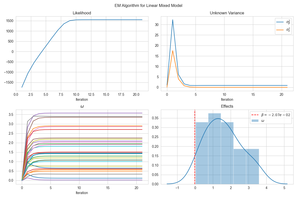
The results below are obtained by running the EM algorithm on a generated dataset.

The results in code are obtained by running the EM algorithm on a given dataset.

TODO:

Acceleration:

1. Aitken acceleration
2. numba

---

1. Notes on the derivation of the posterior distribution of $\mathbf{\beta}$: Let $g(\mathbf{\beta})= -\frac{1}{2}(\mathbf{y} - \mathbf{Z}\mathbf{\omega} - \mathbf{X}\mathbf{\beta})^T (\sigma_e^2\mathbf{I}_n)^{-1} (\mathbf{y} - \mathbf{Z}\mathbf{\omega} - \mathbf{X}\mathbf{\beta}) -\frac{1}{2} \mathbf{\beta}^T (\sigma_\beta^2 \mathbf{I}_p)^{-1} \mathbf{\beta}$. Then we have $\nabla g(\mathbf{\beta}) = \mathbf{X}^T (\mathbf{y} - \mathbf{Z}\mathbf{\omega} - \mathbf{X}\mathbf{\beta})/\sigma_e^2 - \mathbf{\beta}/\sigma_\beta^2$. Let $\nabla g(\mathbf{\beta}) = 0$, we have $\mathbf{\beta} = \mathbf{\Gamma} \mathbf{X}^T (\mathbf{y} - \mathbf{Z}\mathbf{\omega})/\sigma_e^2$, where $g(\mathbf{\beta})$ is maximized. Thus, we find the $\mathbf{\mu}$. To obtain the variance of $\mathbf{\beta}$, we need to calculate the Hessian matrix of $g(\mathbf{\beta})$ and evaluate it at $\mathbf{\beta} = \mathbf{\mu}$. The Hessian matrix is given by $\nabla^2 g(\mathbf{\beta}) = \mathbf{X}^T \mathbf{X}/\sigma_e^2 + \mathbf{I}_p/\sigma_\beta^2$. Therefore, the variance of $\mathbf{\beta}$ is $\mathbf{\Gamma} = \left(\frac{\mathbf{X}^T \mathbf{X}}{\sigma_e^2} + \frac{\mathbf{I}_p}{\sigma_\beta^2} \right)^{-1}$. ↩︎

2. $\log |\mathbf{\Sigma}|$: Directly calculate the log determinant of $\mathbf{\Sigma}$ would cause numerical overflow:RuntimeWarning: overflow encountered in reduce return ufunc.reduce(obj, axis, dtype, out, **passkwargs) That's because "If an array has a very small or very large determinant, then a call to det may overflow or underflow". When the dimension of $\mathbf{\Sigma}$ is large, $|\mathbf{\Sigma}|$ would be extremely close to zero so that it may be considered as zero by numpy. Therefore, we use $\log |\mathbf{\Sigma}| = \sum_{i=1}^n \log \lambda_i$ to calculate the log determinant of $\mathbf{\Sigma}$. ↩︎

3. When calculating the eigenvalue decomposition, it's better to use 'numpy.linalg.eigh' instead of 'numpy.linalg.eig' since $\tilde{\mathbf{\Gamma}}$ is a real symmetric matrix. The former is faster and more accurate than the latter. ↩︎