A survey on deep learning image classification technics based on PyTorch and PyTorch lightning

Zhang Yuxuan, Jiang Wenxin, Fan Yifei, Zhang Juntao (In order of speakers)

Contents

1. Image Generation
2. Training and Tuning with Tricks
3. Graph Attention ViT
4. Interpretion

Data Augmentation: Image Generation

• Increasing model's ability to generalize to new and unseen data.
• Help the model learn more robust and invariant features.

DCGAN

Diffusion Model

• Foward process

$$ q\left(x_t \mid x_{t-1}\right)=\mathcal{N}\left(x_t ; \sqrt{1-\beta_t} x_{t-1}, \beta_t \mathbf{I}\right) $$$$ q\left(x_{1: T} \mid x_0\right)=\prod_{t=1}^T q\left(x_t \mid x_{t-1}\right) $$

• Reverse process

$$ p_\theta\left(x_{0: T}\right)=p\left(x_T\right) \prod_{t=1}^T p_\theta\left(x_{t-1} \mid x_t\right) $$$$ p_\theta\left(x_{t-1} \mid x_t\right)=\mathcal{N}\left(x_{t-1} ; \mu_\theta\left(x_t, t\right), \Sigma_\theta\left(x_t, t\right)\right) $$

• loss

$$ L_t^{\text {simple }} = \mathbb{E}_ {t \sim [1,T] , \mathbf{x}_ {0}, \boldsymbol{\epsilon}_ {t}} \left[||\boldsymbol{\epsilon}_ t-\boldsymbol{\epsilon}_ \theta\left(\sqrt{\bar{\alpha}_ t} \mathbf{x}_ 0+\sqrt{1-\bar{\alpha}_ t} \boldsymbol{\epsilon}_ t, t\right)||^2 \right] $$

Generated Dataset

Training and Tuning with Tricks for CIFAR-10 dataset in PyTorch and PyTorch Lightning

Jiang Wenxin

• Easy convert

• Less code, more efficient.

callbacks = [
    ModelCheckpoint(monitor="val_acc", mode="max"),
    LearningRateMonitor(logging_interval="step"),
    StochasticWeightAveraging(swa_lrs=1e-2),
    early_stopping,
]
trainer = Trainer(
    max_epochs=50,
    devices='auto', # auto choose GPU or CPU
    logger=wandb_logger,
    callbacks=callbacks, # defined above
)

Datasets and models

• Dataset: CIFAR-10
• Model: ResNet18 or ResNet34 from TorchVision.Models
• Loss Function: NLL(Negative Log-Likelihood)
• Optimizer: SGD(Stochastic Gradient Descent) or Adam(Adaptive Moment Estimation)
• Hyperparameters: Learning Rate, Batch Size, Schedule, etc.

Transforms: Data Augmentation

Tools: random crop, random flip, random rotation, etc. Benefits of data augmentation:

• Increase the size of the dataset -> Reduce overfitting
• Improve generalization -> Improve the performance of the model
• Increase at least 3% accuracy in CIFA-10$^1$

Transforms: Data Normalization and Resizing

Tools: Normalize, Resize, etc. Why data normalization?

• Easier to converge
• Prevent gradient explosion / vanish
• Make features have the same scale

Why data resizing?

• Reduce the size of the img -> Save time
• Fit the size of input layer

Transfer Learning

• Use the pretrained model to initialize the weights of the model

model = torchvision.models.resnet18(pretrained=True)

Useful when dataset is small.

Replicability and Determinism

# for hardware
torch.backends.cudnn.deterministic = True
torch.backends.cudnn.benchmark = False
# for numpy/pytorch package
seed_everything(42)

Tricks: Learning Rate Finder

(But it sometimes doesn't work well.) Not to pick the lowest loss, but in the middle of the sharpest downward slope (red point).

Effective Training Techniques

callbacks = [
    LearningRateMonitor(logging_interval="step"),
    StochasticWeightAveraging(swa_lrs=1e-2),
    GradientAccumulationScheduler(scheduling={...}),
    early_stopping
]

trainer = Trainer(
    gradient_clip_val=0.5,
    devices='auto',  # default
    logger=wandb_logger,...
)

• Accumulate Gradients:

Accumulated gradients run K small batches of size N before doing a backward pass, resulting a KxN effective batch size. Control batch size, improve the stability and generalisation of the model

• Early Stopping:

Stop at the best epoch, not the last epoch. Avoid over-fitting.

• Gradient Clipping:

Gradient clipping can be enabled to avoid exploding gradients.

• Stochastic Weight Averaging:

Smooths the loss landscape thus making it harder to end up in a local minimum during optimization. Improves generalization.

• Learning Rate Scheduler:

Control learning rate. Make the model converge faster.

• Manage Experiment: Weights and Biases: WandB

Before training: After training:

• Manage Experiment: Weights and Biases: WandB

Dashboard: Or more commonly used: TensorBoard

Results

Graph Attention ViT

In pratice, since the transformer becomes more and more popular, many companies and researchers want to add attention block to their existed model in order to improve the performance. However, training an attention related model is computation consuming and not easy.

In this project, we add the attention block to the resnet18 model. And we follow the ViT structure to utilize the attention block.

The basis of attention

• The general form for the self-attention

  $$ A_{ij}=f(h_i,h_j) $$

  where $h_i$ and $h_j$ are the features for node $i$ and $j$, and $f$ is an arbitrary function that computes the attention score between two nodes.

• The classical self-attention

  $$ A=softmax\left(\frac{H^{\top}(Q^{\top}K)H}{\sqrt{d_k}}\right) $$

  where $H\in\mathbb{R}^{f\times n}$ is the feature matrix for each embedding, $Q,K\in\mathbb{R}^{f^{'}\times f}$ are the query and key matrix for self-attention, and $d_k$ is the dimension of the key vector. Actually, it's just a bilinear function.

Graph Attention Block

The graph attention block is shown in the following figure,

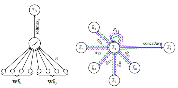
• The formula for graph attention

  $$ A_{ij}=softmax(\sigma(W^{\top}[h_i||h_j])) $$

  where $W\in\mathbb{R}^{f\times 1}$ is the weight, $h_i\in \mathbb{R}^{f}$ is the feature of the $i^{th}$ node and $\sigma$ represents for activation function.

Graph Attention Block

Convert in this form, the attention matrix $A$ can be computed as follows:

$$ A=softmax(\sigma(W_K^{\top}H+H^{\top}W_Q)) $$

where $H\in\mathbb{R}^{f\times n}$ is the feature matrix of all nodes.

Then we can implement the graph attention block in pytorch like this:

Q = H @ W_Q
# Q : (batch, nodes, 1)
K = H @ W_K
# K : (batch, nodes, 1)
A = torch.softmax(self.activation(Q.transpose(-1,-2)+K),dim=-1)
# A : (batch, nodes, nodes)

Conv2d Embedding

In order to use the graph attention block, we should convert patches into feature vectors of nodes in the graph. In this project, we use the Conv2d layer to convert instead of the Flatten layer.

nn.Conv2d(chans,feats,kernel_size=patch_size,stride=patch_size)

Set the kernel_size and stride_size equal to patch_size.

Experiment

Model	Pretrained	Attention	Epoch Consuming	Test Accuracy
Resnet18			50	0.926
Resnet18 + GraphAtten		✔️	50	0.918
Resnet18 |> GraphAtten	✔️	✔️	5	0.935
Resnet18 |> ClassicAtten	✔️	✔️	5	0.931

The test accuracy even decreases when we add the attention block to the resnet18 model and train whole model from the begining. However, when we use the pretrained model, the metric increases.

Conclusion

In conclusion, using the pretrained model to boost the performance of new added attention block is a good choice.

Here are the advantages of this method:

1. Don't need to train the whole model from the beginning. It's easy to just train a new added block.
2. Improve the performance of the existed model just in a few epochs, saving time and money.

Model interpretability on CIFAR-10

Apply model interpretability algorithms from Captum library on CIFAR-10 dataset in order to attribute the label of the image to the input pixels and visualize it.

• Display the original image
• Compute gradients with respect to its class and transposes them for visualization purposes.
• Apply integrated gradients attribution algorithm to computes the integral of the gradients of the output prediction for its class with respect to the input image pixels.
• Use integrated gradients and noise tunnel with smoothgrad square option on the test image. Add gaussian noise to the input image $n$ times, computes the attributions for $n$ images and returns the mean of the squared attributions across $n$ images.
• Apply DeepLift on test image. Deeplift assigns attributions to each input pixel by looking at the differences of output and its reference in terms of the differences of the input from the reference.

$$ \text { IntegratedGrads }_i(x)::=\left(x_i-x_i^{\prime}\right) \times \int_{\alpha=0}^1 \frac{\partial F\left(x^{\prime}+\alpha \times\left(x-x^{\prime}\right)\right)}{\partial x_i} d \alpha $$

Results of "cat" class:

Results of "plane" class:

Results of "ship" class:

Results of "ship" class:

Then, we apply model interpretability algorithms with a handpicked image and visualizes the attributions for each pixel by overlaying them on the image.

• Integrated gradients smoothened by a noise tunnel.

• GradientShap, a linear explanation model which uses a distribution of reference samples to explain predictions of the model.

• Occlusion-based attribution method to estimate which areas of the image are critical for the classifier's decision by occluding them and quantifying how the decision changes.

Collaboration with Git and Colab

Git is an open source distributed version control system for teams or individuals to handle projects quickly and efficiently. And colab is a free cloud service and supports free GPUs. It is a good choice for us to use git and colab to collaborate on the project, we managed the project and shared the code easily and efficiently in the teamwork.

Reference

1. Shorten C, Khoshgoftaar T M. A survey on image data augmentation for deep learning[J]. Journal of big data, 2019, 6(1): 1-48.
2. PyTorch Lightning: https://lightning.ai/docs/pytorch/stable/
3. PyTorch Lightning CIFAR-10: https://lightning.ai/docs/pytorch/stable/notebooks/lightning_examples/cifar10-baseline.html
4. Training tricks: https://lightning.ai/docs/pytorch/stable/advanced/training_tricks.html

Reference

5. Graph Attention: https://www.baeldung.com/cs/graph-attention-networks
6. Diffusion Model:https://lilianweng.github.io/posts/2021-07-11-diffusion-models/#:~:text=Diffusion%20models%20are%20inspired%20by,data%20samples%20from%20the%20noise
7. Cifar-10 Generation with Diffusion Model:https://github.com/zoubohao/DenoisingDiffusionProbabilityModel-ddpm-
8. Axiomatic Attribution for Deep Networks:https://arxiv.org/pdf/1703.01365.pdf

Thanks for your listening!