# install.packages("susieR")
# install.packages("Rfast")SusieR Examples
Minimal Example
library(susieR)
set.seed(1)
n <- 1000
p <- 1000
beta <- rep(0, p)
beta[c(1, 2, 300, 400)] <- 1
X_ <- matrix(rnorm(n * p), nrow = n, ncol = p)
y <- X_ %*% beta + rnorm(n)
res <- susie(X_, y, L = 10)
plot(coef(res)[-1], pch = 20)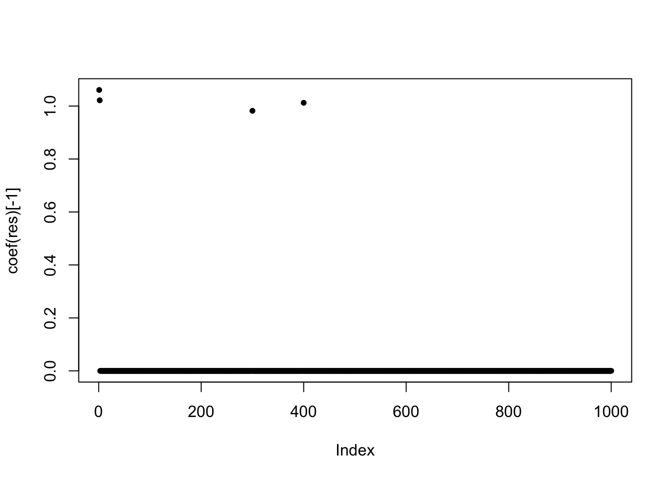
plot(y, predict(res), pch = 20)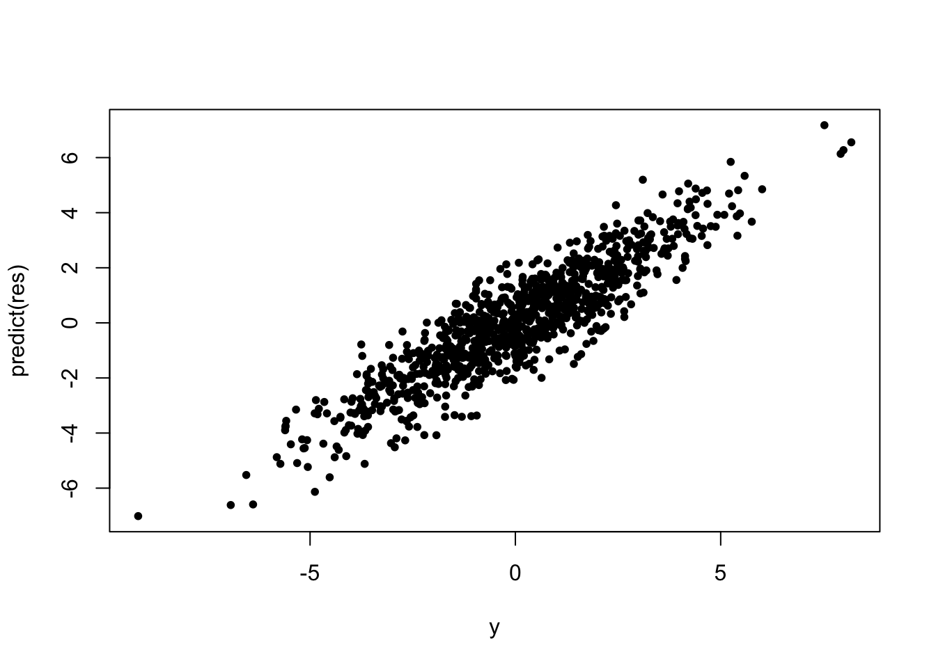
Fine-mapping Example
Notice that we’ve simulated 2 sets of \(Y\) as 2 simulation replicates. Here we’ll focus on the first data-set.
data(N3finemapping)
attach(N3finemapping)
X <- N3finemapping$X
Y <- N3finemapping$Y
Here are the 3 “true” signals in the first data-set:
b <- true_coef[, 1]
which(b != 0)
[1] 403 653 773plot(b, pch = 16, ylab = "effect size")
Simple regression summary statistics
univariate_regression function can be used to compute summary statistics by fitting univariate simple regression variable by variable. The results are \(\hat{\beta}\) and \(SE(\hat{\beta})\) from which z-scores can be derived. Again we focus only on results from the first data-set:
sumstats <- univariate_regression(X, Y[, 1])
z_scores <- sumstats$betahat / sumstats$sebetahat
susie_plot(z_scores, y = "z", b = b)
title("z-scores from univariate regression")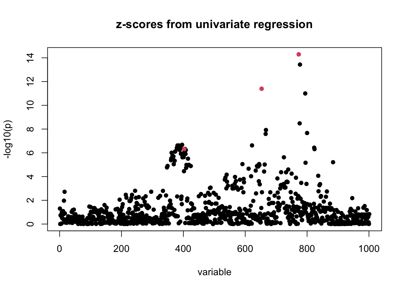
Fine-mapping with susieR
For starters, we assume there are at most 10 causal variables, i.e., set L = 10, although SuSiE is robust to the choice of L.
The susieR function call is:
fitted <- susie(X, Y[, 1],
    L = 10,
    verbose = TRUE
)
[1] "objective:-1380.57545244545"
[1] "objective:-1377.48660917471"
[1] "objective:-1375.85777207681"
[1] "objective:-1375.8089230143"
[1] "objective:-1370.339493334"
[1] "objective:-1370.19677277366"
[1] "objective:-1370.1091973921"
[1] "objective:-1370.10918017476"
[1] "objective:-1370.10901872279"Credible sets
By default, we output 95% credible set:
print(fitted$sets)$cs
$cs$L2
[1] 653
$cs$L1
[1] 773 777
$cs$L3
[1] 362 365 372 373 374 379 381 383 384 386 387 388 389 391 392 396 397 398 399
[20] 400 401 403 404 405 407 408 415
$purity
min.abs.corr mean.abs.corr median.abs.corr
L2 1.0000000 1.0000000 1.0000000
L1 0.9815726 0.9815726 0.9815726
L3 0.8686309 0.9640176 0.9720711
$cs_index
[1] 2 1 3
$coverage
[1] 0.9998236 0.9988858 0.9539811
$requested_coverage
[1] 0.95The 3 causal signals have been captured by the 3 CS reported here. The 3rd CS contains many variables, including the true causal variable 403. The minimum absolute correlation is 0.86.
If we use the default 90% coverage for credible sets, we still capture the 3 signals, but “purity” of the 3rd CS is now 0.91 and size of the CS is also a bit smaller.
sets <- susie_get_cs(fitted,
    X = X,
    coverage = 0.9,
    min_abs_corr = 0.1
)print(sets)$cs
$cs$L2
[1] 653
$cs$L1
[1] 773 777
$cs$L3
[1] 373 374 379 381 383 384 386 387 388 389 391 392 396 398 399 400 401 403 404
[20] 405 407 408
$purity
min.abs.corr mean.abs.corr median.abs.corr
L2 1.0000000 1.0000000 1.0000000
L1 0.9815726 0.9815726 0.9815726
L3 0.9119572 0.9726283 0.9765888
$cs_index
[1] 2 1 3
$coverage
[1] 0.9998236 0.9988858 0.9119917
$requested_coverage
[1] 0.9Posterior inclusion probabilities
Previously we’ve determined that summing over 3 single effect regression models is approperate for our application. Here we summarize the variable selection results by posterior inclusion probability (PIP):
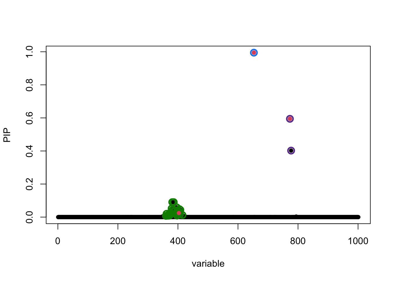
susie_plot(fitted, y = "PIP", b = b)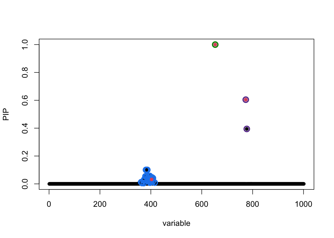
The true causal variables are colored red. The 95% CS identified are circled in different colors. Of interest is the cluster around position 400. The true signal is 403 but apparently it does not have the highest PIP. To compare ranking of PIP and original z-score in that CS:
i <- fitted$sets$cs[[3]]
z3 <- cbind(i, z_scores[i], fitted$pip[i])
colnames(z3) <- c("position", "z-score", "PIP")
z3[order(z3[, 2], decreasing = TRUE), ]
position z-score PIP
[1,] 396 5.189811 0.056704331
[2,] 381 5.164794 0.100360243
[3,] 386 5.164794 0.100360243
[4,] 379 5.077563 0.054179507
[5,] 391 5.068388 0.055952118
[6,] 383 5.057053 0.052896918
[7,] 384 5.057053 0.052896918
[8,] 389 5.052519 0.042161265
[9,] 405 5.039617 0.045761975
[10,] 403 5.035949 0.031992848
[11,] 387 5.013526 0.041041505
[12,] 388 4.997955 0.039650079
[13,] 408 4.994865 0.041551961
[14,] 404 4.954407 0.032013339
[15,] 374 4.948060 0.030571484
[16,] 373 4.934410 0.023577221
[17,] 362 4.894243 0.012145481
[18,] 399 4.860780 0.026454056
[19,] 392 4.856384 0.019741011
[20,] 407 4.849285 0.014699313
[21,] 400 4.827361 0.021659443
[22,] 365 4.782770 0.006263425
[23,] 398 4.751205 0.012907848
[24,] 401 4.723184 0.014858460
[25,] 397 4.716886 0.008690915
[26,] 415 4.663208 0.009003129
[27,] 372 4.581560 0.005886458Choice of priors
Notice that by default SuSiE estimates prior effect size from data. For fine-mapping applications, however, we sometimes have knowledge of SuSiE prior effect size since it is parameterized as percentage of variance explained (PVE) by a non-zero effect, which, in the context of fine-mapping, is related to per-SNP heritability. It is possible to use scaled_prior_variance to specify this PVE and explicitly set estimate_prior_variance=FALSE to fix the prior effect to given value.
In this data-set, SuSiE is robust to choice of priors. Here we set PVE to 0.2, and compare with previous results:
fitted <- susie(X, Y[, 1],
    L = 10,
    estimate_residual_variance = TRUE,
    estimate_prior_variance = FALSE,
    scaled_prior_variance = 0.2
)
susie_plot(fitted, y = "PIP", b = b)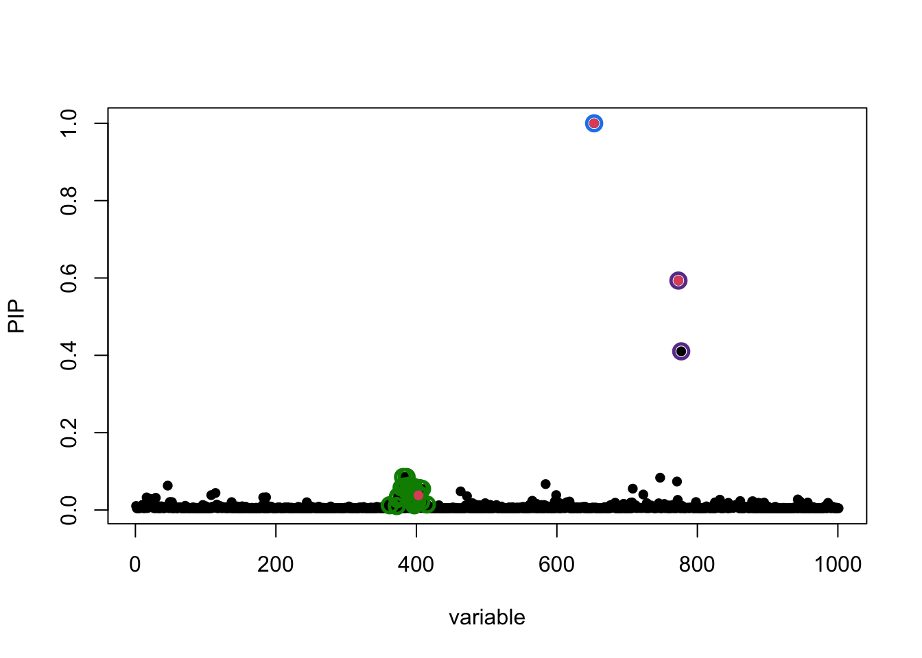
which largely remains unchanged.
A note on covariate adjustment
To include covariate Z in SuSiE, one approach is to regress it out from both y and X, and then run SuSiE on the residuals. The code below illustrates the procedure:
remove.covariate.effects <- function(X, Z, y) {
    # include the intercept term
    if (any(Z[, 1] != 1)) Z <- cbind(1, Z)
    A <- forceSymmetric(crossprod(Z))
    SZy <- as.vector(solve(A, c(y %*% Z)))
    SZX <- as.matrix(solve(A, t(Z) %*% X))
    y <- y - c(Z %*% SZy)
    X <- X - Z %*% SZX
    return(list(X = X, y = y, SZy = SZy, SZX = SZX))
}

out <- remove.covariate.effects(X, Z, Y[, 1])
fitted_adjusted <- susie(out$X, out$y, L = 10)
Note that the covariates Z should have a column of ones as the first column. If not, the above function remove.covariate.effects will add such a column to Z before regressing it out. Data will be centered as a result. Also the scale of data is changed after regressing out Z. This introduces some subtleties in terms of interpreting the results. For this reason, we provide covariate adjustment procedure as a tip in the documentation and not part of susieR::susie() function. Cautions should be taken when applying this procedure and interpreting the result from it.
Fine-mapping with Summary Data
The data-set
data(N3finemapping)
attach(N3finemapping)
The following objects are masked _by_ .GlobalEnv:
X, YThe following objects are masked from N3finemapping (pos = 3):
allele_freq, chrom, pos, residual_variance, true_coef, V, X, Yn <- nrow(X)Notice that we’ve simulated two sets of \(Y\) as two simulation replicates. Here we’ll focus on the first data-set.
dim(Y)[1] 574 2Here are the three true signals in the first data-set:
b <- true_coef[, 1]
plot(b, pch = 16, ylab = "effect size")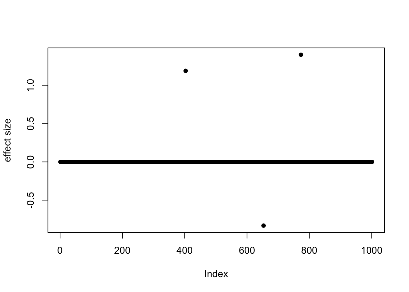
which(b != 0)[1] 403 653 773So the underlying causal variables are 403, 653 and 773.
Summary statistics from simple regression
Summary statistics of genetic association studies typically contain effect sizes (\(\hat{\beta}\) coefficient from regression) and p-values. These statisticscan be used to perform fine-mapping with given an additional input of correlation matrix between variables. The correlation matrix in genetics is typically referred to as an “LD matrix” (LD is short for linkage disequilibrium). One may use external reference panels to estimate it when this matrix cannot be obtained from samples directly. Importantly, the LD matrix has to be a matrix containing estimates of the correlation, \(r\), and not \(r^2\) or \(|r|\). See also this vignette for how to check the consistency of the LD matrix with the summary statistics.
The univariate_regression function can be used to compute summary statistics by fitting univariate simple regression variable by variable. The results are \(\hat{\beta}\) and \(SE(\hat{\beta})\) from which z-scores can be derived. Alternatively, you can obtain z-scores from \(\hat{\beta}\) and p-values if you are provided with those information. For example,
sumstats <- univariate_regression(X, Y[, 1])
z_scores <- sumstats$betahat / sumstats$sebetahat
susie_plot(z_scores, y = "z", b = b)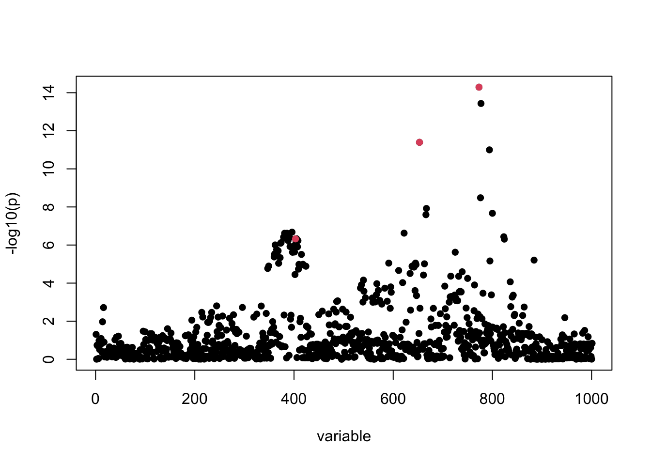
For this example, the correlation matrix can be computed directly from data provided:
R <- cor(X)Fine-mapping with susieR using summary statistics
By default, SuSiE assumes at most 10 causal variables, with L = 10, although we note that SuSiE is generally robust to the choice of L.
Since the individual-level data is available for us here, we can easily compute the “in-sample LD” matrix, as well as the variance of \(y\), which is 7.8424. (By “in-sample”, we means the LD was computed from the exact same matrix X that was used to obtain the other statistics.) When we fit SuSiE regression with summary statistics, \(\hat{\beta}\), \(SE(\hat{\beta})\), \(R\), \(n\), and var_y these are also the sufficient statistics. With an in-sample LD, we can also estimate the residual variance using these sufficient statistics. (Note that if the covariate effects are removed from the genotypes in the univariate regression, it is recommended that the “in-sample” LD matrix also be computed from the genotypes after the covariate effects have been removed.)
fitted_rss1 <- susie_rss(
    bhat = sumstats$betahat, shat = sumstats$sebetahat, n = n, R = R, var_y = var(Y[, 1]), L = 10,
    estimate_residual_variance = TRUE
)
HINT: For estimate_residual_variance = TRUE, please check that R is the "in-sample" LD matrix; that is, the correlation matrix obtained using the exact same data matrix X that was used for the other summary statistics. Also note, when covariates are included in the univariate regressions that produced the summary statistics, also consider removing these effects from X before computing R.Using summary, we can examine the posterior inclusion probability (PIP) for each variable, and the 95% credible sets:
summary(fitted_rss1)$cs cs cs_log10bf cs_avg_r2 cs_min_r2
1 2 4.033879 1.0000000 1.0000000
2 1 6.744086 0.9634847 0.9634847
3 3 3.461470 0.9293299 0.7545197
variable
1 653
2 773,777
3 362,365,372,373,374,379,381,383,384,386,387,388,389,391,392,396,397,398,399,400,401,403,404,405,407,408,415The three causal signals have been captured by the three CSs. Note the third CS contains many variables, including the true causal variable 403.
We can also plot the posterior inclusion probabilities (PIPs):
susie_plot(fitted_rss1, y = "PIP", b = b)
The true causal variables are shown in red. The 95% CSs are shown by three different colours (green, purple, blue).
Note this result is exactly the same as running susie on the original individual-level data:
fitted <- susie(X, Y[, 1], L = 10)
all.equal(fitted$pip, fitted_rss1$pip)
[1] TRUEall.equal(coef(fitted)[-1], coef(fitted_rss1)[-1])[1] TRUEIf, on the other hand, the variance of \(y\) is unknown, we fit can SuSiE regression with summary statistics, \(\hat{\beta}\), \(SE(\hat{\beta})\), \(R\) and \(n\) (or z-scores, \(R\) and \(n\)). The outputted effect estimates are now on the standardized \(X\) and \(y\) scale. Still, we can estimate the residual variance because we have the in-sample LD matrix:
fitted_rss2 <- susie_rss(
    z = z_scores, R = R, n = n, L = 10,
    estimate_residual_variance = TRUE
)
HINT: For estimate_residual_variance = TRUE, please check that R is the "in-sample" LD matrix; that is, the correlation matrix obtained using the exact same data matrix X that was used for the other summary statistics. Also note, when covariates are included in the univariate regressions that produced the summary statistics, also consider removing these effects from X before computing R.The result is same as if we had run susie on the individual-level data, but the output effect estimates are on different scale:
all.equal(fitted$pip, fitted_rss2$pip)[1] TRUEplot(coef(fitted)[-1], coef(fitted_rss2)[-1], xlab = "effects from SuSiE", ylab = "effects from SuSiE-RSS", xlim = c(-1, 1), ylim = c(-0.3, 0.3))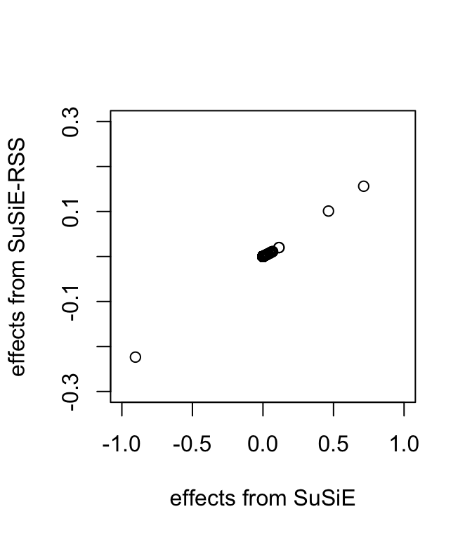
Specifically, without the variance of \(y\), these estimates are same as if we had applied SuSiE to a standardized \(X\) and \(y\); that is, as if \(y\) and the columns of \(X\) had been normalized so that \(y\) and each column of \(X\) had a standard deviation of 1.
fitted_standardize <- susie(scale(X), scale(Y[, 1]), L = 10)
all.equal(coef(fitted_standardize)[-1], coef(fitted_rss2)[-1])
[1] TRUEFine-mapping with susieR using LD matrix from reference panel
When the original genotypes are not available, one may use a separate reference panel to estimate the LD matrix.
To illustrate this, we randomly generated 500 samples from \(N(0,R)\) and treated them as reference panel genotype matrix X_ref.
We fit the SuSiE regression using out-of sample LD matrix. The residual variance is fixed at 1 because estimating residual variance sometimes produces very inaccurate estimates with out-of-sample LD matrix. The output effect estimates are on the standardized \(X\) and \(y\) scale.
fitted_rss3 <- susie_rss(z_scores, R_ref, n = n, L = 10)susie_plot(fitted_rss3, y = "PIP", b = b)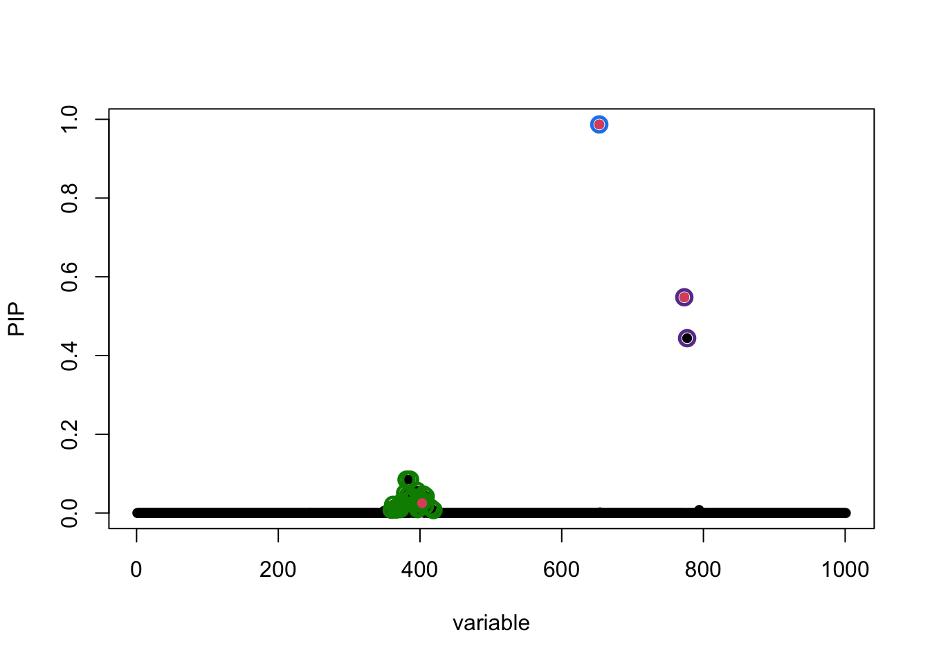
In this particular example, the SuSiE result with out-of-sample LD is very similar to using the in-sample LD matrix because the LD matrices are quite similar.
plot(fitted_rss1$pip, fitted_rss3$pip, ylim = c(0, 1), xlab = "SuSiE PIP", ylab = "SuSiE-RSS PIP")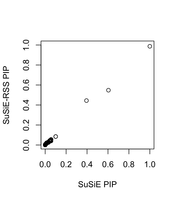
In some rare cases, the sample size \(n\) is unknown. When the sample size is not provided as input to susie_rss, this is in effect assuming the sample size is infinity and all the effects are small, and the estimated PVE for each variant will be close to zero. The outputted effect estimates are on the “noncentrality parameter” scale.
fitted_rss4 <- susie_rss(z_scores, R_ref, L = 10)WARNING: Providing the sample size (n), or even a rough estimate of n, is highly recommended. Without n, the implicit assumption is n is large (Inf) and the effect sizes are small (close to zero).susie_plot(fitted_rss4, y = "PIP", b = b)