Notes for XMAP

Key contribution: Propose a statistical method for cross-population fine-mapping common causal SNPs (XMAP) by leveraging genetic diversity (different LD structures) and accounting for confounding bias which addresses the challenges of:

1. Strong linkage disequilibrium among variants can limit the statistical power and resolution of fine-mapping. [Solved by LDSC and SuSiE]
2. Computationally expensive to simultaneously search for multiple causal variants. [Solved by SuSiE]
3. The confounding bias hidden in GWAS summary statistics can produce spurious signals. [Adjusting by the inflation factor $c$]

It also integrates the polygenic component $\boldsymbol{\phi}$ to capture the genetic background effects.

It can be integrated with single cell data to identify trait-relevant cell populations at the single cell resolution.

Advantages over existing methods: Greater statistical power, better calibrate of false positive rate, and substantially higher computational efficiency for identifying multiple causal signals.

Algorithm: Variational expectation-maximization (VEM).

• Notes for XMAP
  • Model and Algorithm
    • XMAP Model for Individual-level Data
    • XMAP Model for Summary-level Data
    • Algorithm and Parameter Estimation
    • Identification of Causal Variant and Construction of Credible Set (Output)
  • Conclusion
    • Simulation Study
    • Real Data Analysis
  • Limitations
  • Reference
  • TO-DO

Model and Algorithm

XMAP Model for Individual-level Data

• Input: GWAS datasets $\left\{\mathbf{y}_1, \mathbf{X}_1\right\}$ and $\left\{\mathbf{y}_2, \mathbf{X}_2\right\}$ from two different populations, where $\mathbf{y}_1 \in \mathbb{R}^{n_1}$ and $\mathbf{y}_2 \in \mathbb{R}^{n_2}$ are phenotype vectors, $\mathbf{X}_1 \in \mathbb{R}^{n_1 \times p}$ and $\mathbf{X}_2 \in$ $\mathbb{R}^{n_2 \times p}$ are genotype matrices, $p$ is the number of SNPs in the locus of interest, and $n_1$ and $n_2$ are the GWAS sample sizes of populations 1 and 2 , respectively. Assume that the columns of $\mathbf{X}_1$ and $\mathbf{X}_2$ have been standardized to have zero mean and unit variance.
• Model:
  • Linear models to relate genotypes and phenotypes:
    $$\begin{equation} \begin{aligned} & \mathbf{y}_1=\mathbf{X}_1 \mathbf{b}_1+\mathbf{X}_1 \boldsymbol{\phi}_1+\mathbf{e}_1, \\ & \mathbf{y}_2=\mathbf{X}_2 \mathbf{b}_2+\mathbf{X}_2 \boldsymbol{\phi}_2+\mathbf{e}_2, \end{aligned}\end{equation}$$
    where $\mathbf{b}_1 \in \mathbb{R}^p$ and $\mathbf{b}_2 \in \mathbb{R}^p$ are sparse vectors of causal effects with major impact on phenotypes, $\boldsymbol{\phi}_1=\left[\phi_{11}, \phi_{12}, \ldots, \phi_{1 p}\right]^T \in \mathbb{R}^p$ and $\boldsymbol{\phi}_2=\left[\phi_{21}, \phi_{22}, \ldots, \phi_{2 p}\right]^T \in \mathbb{R}^p$ are dense vectors capturing the polygenic effects, and $\mathbf{e}_1 \sim \mathcal{N}\left(\mathbf{0}, \sigma_{\mathbf{e}_1}^2 \mathbf{I}_{n_1}\right)$ and $\mathbf{e}_2 \sim \mathcal{N}\left(\mathbf{0}, \sigma_{\mathbf{e}_2}^2 \mathbf{I}_{n_2}\right)$ are vectors of independent noises from populations 1 and 2 , respectively.
  • Decomposition of the causal genetic effects $\mathbf{b}_1$ and $\mathbf{b}_2$ into $K$ 'single effects':
    $$\begin{equation} \begin{align*} & \mathbf{y}_1=\mathbf{X}_1 \sum_{k=1}^K \boldsymbol{\gamma}_k \beta_{1 k}+\mathbf{X}_1 \boldsymbol{\phi}_1+\mathbf{e}_1, \\ & \mathbf{y}_2=\mathbf{X}_2 \sum_{k=1}^K \boldsymbol{\gamma}_k \beta_{2 k}+\mathbf{X}_2 \boldsymbol{\phi}_2+\mathbf{e}_2, \end{align*} \end{equation}$$
    where $\beta_{1 k}$ and $\beta_{2 k}$ are effect sizes of the $k$-th causal signal in populations one and two, respectively, $\boldsymbol{\gamma}_k=\left[\gamma_{k 1}, \ldots, \gamma_{k p}\right]^T \in\{0,1\}^p$ in which only one element is 1 and the rest are 0 with $\gamma_{k j}=1$ indicating the $j$-th variant is responsible for the $k$-th causal signal.
  • Probabilistic structures for the genetic effects:
    $$\begin{equation} \begin{align*} & \boldsymbol{\gamma}_{k} \sim \operatorname{Mult}\left(1,[1 / p, \ldots, 1 / p]^{T}\right), \\ & {\left[\begin{array}{l} \beta_{1 k} \\ \beta_{2 k} \end{array}\right] \sim \mathcal{N}\left(\mathbf{0}, \Sigma_{k}\right), \text { for } k=1, \ldots, K,}\\ & {\left[\begin{array}{l} \phi_{1 j} \\ \phi_{2 j} \end{array}\right] \sim \mathcal{N}(\mathbf{0}, \boldsymbol{\Omega}), \text { for } j=1, \ldots, p,} \end{align*}\end{equation}$$
    where Mult $\left(1,[1 / p, \ldots, 1 / p]^{T}\right)$ denotes the non-informative categorical distribution of class counts drawn with class probabilities given by $1 / p$ for each SNP, $\mathcal{N}\left(\mathbf{0}, \boldsymbol{\Sigma}_{k}\right)$ and $\mathcal{N}(\mathbf{0}, \boldsymbol{\Omega})$ denote the multivariate normal distributions with mean $\mathbf{0}$ and covariance matrices $\boldsymbol{\Sigma}_{k}=\left[\begin{array}{cc}\sigma_{k 1}^{2} & \sigma_{k 12}^{2} \\ \sigma_{k 12}^{2} & \sigma_{k 2}^{2}\end{array}\right]$ and $\boldsymbol{\Omega}=\left[\begin{array}{cc}\omega_{1} & \omega_{12} \\ \omega_{12} & \omega_{2}\end{array}\right]$, respectively.
  • Covariates and adjustment: [shows the equivalence of the model with and without covariates]
    $$\begin{equation} \begin{align*} & \mathbf{y}_{1}=\mathbf{W}_{1} \mathbf{u}_{1}+\mathbf{X}_{1} \sum_{k=1}^{K} \boldsymbol{\gamma}_{k} \beta_{1 k}+\mathbf{X}_{1} \boldsymbol{\Phi}_{1}+\mathbf{e}_{1} \\ & \mathbf{y}_{2}=\mathbf{W}_{2} \mathbf{u}_{2}+\mathbf{X}_{2} \sum_{k=1}^{K} \boldsymbol{\gamma}_{k} \beta_{2 k}+\mathbf{X}_{2} \boldsymbol{\Phi}_{2}+\mathbf{e}_{2} \end{align*}\end{equation}$$
    where $\mathbf{W}_{1} \in \mathbb{R}^{n_{1} \times q_{1}}$ and $\mathbf{W}_{2} \in \mathbb{R}^{n_{2} \times q_{2}}$ are the covariate matrices of populations 1 and 2, respectively, and $\mathbf{u}_{1} \in \mathbb{R}^{q_{1}}$ and $\mathbf{u}_{2} \in \mathbb{R}^{q_{2}}$ are corresponding vectors of covariate effects. To adjust the covariates, we first construct the projection matrices $\mathbf{P}_{1}=\mathbf{I}-\mathbf{W}_{1}\left(\mathbf{W}_{1}^{T} \mathbf{W}_{1}\right)^{-1} \mathbf{W}_{1}^{T}$ and $\mathbf{P}_{2}=\mathbf{I}-\mathbf{W}_{2}\left(\mathbf{W}_{2}^{T} \mathbf{W}_{2}\right)^{-1} \mathbf{W}_{2}^{T}$. Then we multiply $\mathbf{P}_{1}$ on both sides of the first equation and $\mathbf{P}_{2}$ on both sides of the second equation in model (4). Through this projection, we can obtain a model without covariates:
    $$\begin{equation} \begin{align*} & \mathbf{y}_{1}^{\mathbf{P}}=\mathbf{X}_{1}^{\mathbf{P}} \sum_{k=1}^{K} \boldsymbol{\gamma}_{k} \beta_{1 k}+\mathbf{X}_{1}^{\mathbf{P}} \boldsymbol{\Phi}_{1}+\mathbf{e}_{1}^{\mathbf{P}} \\ & \mathbf{y}_{2}^{\mathbf{P}}=\mathbf{X}_{2}^{\mathbf{P}} \sum_{k=1}^{K} \boldsymbol{\gamma}_{k} \beta_{2 k}+\mathbf{X}_{2}^{\mathbf{P}} \boldsymbol{\phi}_{2}+\mathbf{e}_{2}^{\mathbf{P}} \end{align*}\end{equation}$$
    where $\mathbf{y}_{1}^{\mathbf{P}}=\mathbf{P}_{1} \mathbf{y}_{1}, \quad \mathbf{y}_{2}^{\mathbf{P}}=\mathbf{P}_{2} \mathbf{y}_{2}, \quad \mathbf{X}_{1}^{\mathbf{P}}=\mathbf{P}_{1} \mathbf{X}_{1}, \quad \mathbf{X}_{2}^{\mathbf{P}}=\mathbf{P}_{2} \mathbf{X}_{2}, \quad \mathbf{e}_{1}^{\mathbf{P}}=\mathbf{P}_{1} \mathbf{e}_{1}$, and $\mathbf{e}_{2}^{\mathbf{P}}=\mathbf{P}_{2} \mathbf{e}_{2}$. As we can observe, model (5) reduces to model (2). With this equivalence, we can work with model (2) without loss of generality.

XMAP Model for Summary-level Data

• Input:
  • Summary-level GWAS data $\left\{\hat{\mathbf{b}}_{1}, \hat{\mathbf{s}}_{1}\right\}=\left\{\hat{b}_{1 j}, \hat{s}_{1 j}\right\}_{j=1, \ldots, p}$ and $\left\{\hat{\mathbf{b}}_{2}, \hat{\mathbf{s}}_{2}\right\}=\left\{\hat{b}_{2 j}, \hat{s}_{2 j}\right\}_{j=1, \ldots, p}$ obtained from simple linear regressions:
    $$\begin{equation} \begin{aligned} & \hat{b}_{1 j}=\mathbf{x}_{1 j}^{T} \mathbf{y}_{1} / \mathbf{x}_{1 j}^{T} \mathbf{x}_{1 j}, & \hat{s}_{1 j}=\sqrt{\left\|\mathbf{y}_{1}-\mathbf{x}_{1 j} \hat{b}_{1 j}\right\|_{2}^{2} /\left(n_{1} \mathbf{x}_{1 j}^{T} \mathbf{x}_{1 j}\right)}, \\ & \hat{b}_{2 j}=\mathbf{x}_{2 j}^{T} \mathbf{y}_{2} / \mathbf{x}_{2 j}^{T} \mathbf{x}_{2 j}, & \hat{s}_{2 j}=\sqrt{\left\|\mathbf{y}_{2}-\mathbf{x}_{2 j} \hat{b}_{2 j}\right\|_{2}^{2} /\left(n_{2} \mathbf{x}_{2 j}^{T} \mathbf{x}_{2 j}\right)}, \end{aligned}\end{equation}$$
    where $\mathbf{x}_{1 j} \in \mathbb{R}^{p}$ and $\mathbf{x}_{2 j} \in \mathbb{R}^{p}$ denote the $j$-th column of $\mathbf{X}_{1}$ and $\mathbf{X}_{2}$, respectively.
  • LD matrices $\mathbf{R}_{1}=\left\{r_{1 j l}\right\} \in \mathbb{R}^{p \times p}$ and $\mathbf{R}_{2}=\left\{r_{2 j l}\right\} \in \mathbb{R}^{p \times p}$, where $r_{1 j l}=\mathbb{E}\left[\mathbf{x}_{1 j}^{T} \mathbf{x}_{1 l} / n_{1}\right]$ and $r_{2 j l}=\mathbb{E}\left[\mathbf{x}_{2 j}^{T} \mathbf{x}_{2 l} / n_{2}\right]$ denote the correlation between variants $j$ and $l$ in populations 1 and 2, respectively. The SNP correlation matrices $\mathbf{R}=\left\{\mathbf{R}_{1}, \mathbf{R}_{2}\right\}$ can be estimated with genotypes either from subsets of GWAS samples or from population-matched reference panels.
• Model:
  • Expectation of GWAS effect sizes conditional on $\mathbf{b}$ and $\boldsymbol{\phi}$:
    $$\begin{equation} \begin{aligned} & \mathbb{E}\left[\hat{\mathbf{b}}_{1} \mid \mathbf{b}_{1}, \boldsymbol{\phi}_{1}\right] =\mathbf{R}_{1} \sum_{k=1}^{K} \boldsymbol{\gamma}_{k} \beta_{1 k}+\mathbf{R}_{1} \boldsymbol{\phi}_{1}, \\ & \mathbb{E}\left[\hat{\mathbf{b}}_{2} \mid \mathbf{b}_{2}, \boldsymbol{\phi}_{2}\right] =\mathbf{R}_{2} \sum_{k=1}^{K} \boldsymbol{\gamma}_{k} \beta_{2 k}+\mathbf{R}_{2} \boldsymbol{\phi}_{2} \end{aligned}\end{equation}$$
    Note: $\mathbb{E}\left[\hat{\mathbf{b}} \mid \dots \right]=\mathbb{E}\left[\mathbf{X}^{T} \mathbf{y} / \mathbf{X}^{T} \mathbf{X} \mid \dots \right], \mathbf{X}^{T} \mathbf{X} =1$.
  • Distribution of $\hat{\mathbf{b}}$: Assuming normal distributions for $\hat{\mathbf{b}}_{1}$ and $\hat{\mathbf{b}}_{2}$, we have:
    $$\begin{equation}\begin{align*} & \hat{\mathbf{b}}_{1} \sim \mathcal{N}\left(\mathbf{R}_{1} \sum_{k=1}^{K} \boldsymbol{\gamma}_{k} \beta_{1 k}+\mathbf{R}_{1} \boldsymbol{\Phi}_{1}, \hat{\mathbf{S}}_{1} \mathbf{R}_{1} \hat{\mathbf{S}}_{1}\right), \\ & \hat{\mathbf{b}}_{2} \sim \mathcal{N}\left(\mathbf{R}_{2} \sum_{k=1}^{K} \boldsymbol{\gamma}_{k} \beta_{2 k}+\mathbf{R}_{2} \boldsymbol{\Phi}_{2}, \hat{\mathbf{S}}_{2} \mathbf{R}_{2} \hat{\mathbf{S}}_{2}\right). \end{align*}\end{equation}$$
    where $\hat{\mathbf{S}}_{1} \in \mathbb{R}^{p \times p}$ and $\hat{\mathbf{S}}_{2} \in \mathbb{R}^{p \times p}$ are diagonal matrices with diagonal terms given as $\left\{\hat{\mathbf{S}}_{1}\right\}_{j j}=\hat{s}_{1 j}$ and $\left\{\hat{\mathbf{S}}_{2}\right\}_{j j}=\hat{s}_{2 j}$ for $j=1, \ldots, p$. And $\hat{\mathbf{S}}_{1}\mathbf{R}\hat{\mathbf{S}}_{1}$ and $\hat{\mathbf{S}}_{2}\mathbf{R}\hat{\mathbf{S}}_{2}$ are the variances of $\hat{\mathbf{\epsilon}}_{1}= \hat{\mathbf{X}}_{1}^T\hat{\mathbf{e}}_{1}$ and $\hat{\mathbf{\epsilon}}_{2}= \hat{\mathbf{X}}_{2}^T\hat{\mathbf{e}}_{2}$, respectively.
  • Account for confounding bias: Modify (8) to account for the unadjusted confounding bias:
    $$\begin{equation}\begin{align*} & \hat{\mathbf{b}}_{1} \sim \mathcal{N}\left(\mathbf{R}_{1} \sum_{k=1}^{K} \boldsymbol{\gamma}_{k} \beta_{1 k}+\mathbf{R}_{1} \boldsymbol{\Phi}_{1}, c_{1} \hat{\mathbf{S}}_{1} \mathbf{R}_{1} \hat{\mathbf{S}}_{1}\right), \\ & \hat{\mathbf{b}}_{2} \sim \mathcal{N}\left(\mathbf{R}_{2} \sum_{k=1}^{K} \boldsymbol{\gamma}_{k} \beta_{2 k}+\mathbf{R}_{2} \boldsymbol{\Phi}_{2}, c_{2} \hat{\mathbf{S}}_{2} \mathbf{R}_{2} \hat{\mathbf{S}}_{2}\right). \end{align*}\end{equation}$$
    where $c_{1}$ and $c_{2}$ are LDSC intercepts that indicate the magnitude of inflation in GWAS effect sizes due to confounding bias. In the absence of confounding bias, the values of inflation constants $c_{1}$ and $c_{2}$ are close to one.

Algorithm and Parameter Estimation

Denote the collection of unknown parameters $\boldsymbol{\theta}=\left\{\boldsymbol{\Sigma}, \boldsymbol{\Omega}, c_{1}, c_{2}\right\}$, and the collections of latent variables $\boldsymbol{\phi}=\left\{\boldsymbol{\phi}_{1}, \boldsymbol{\phi}_{2}\right\}, \boldsymbol{\gamma}=\left\{\boldsymbol{\gamma}_{k}\right\}_{k=1, \ldots, K}$ and $\boldsymbol{\beta}=\left\{\beta_{1 k}, \beta_{2 k}\right\}_{k=1, \ldots, K}$. Obtain the parameter estimates $\boldsymbol{\theta}$ and identify causal SNPs with the posterior:
$$\begin{equation} \operatorname{Pr}(\boldsymbol{\gamma}, \boldsymbol{\beta}, \boldsymbol{\Phi} \mid \hat{\mathbf{b}}, \hat{\mathbf{s}}, \mathbf{R} ; \hat{\boldsymbol{\theta}})=\frac{\operatorname{Pr}(\hat{\mathbf{b}}, \boldsymbol{\gamma}, \boldsymbol{\beta}, \boldsymbol{\phi} \mid \hat{\mathbf{s}}, \mathbf{R} ; \hat{\boldsymbol{\theta}})}{\operatorname{Pr}(\hat{\mathbf{b}} \mid \hat{\mathbf{s}}, \mathbf{R} ; \hat{\boldsymbol{\theta}})}. \end{equation}$$

1. First step: Apply LDSC to estimate the parameters $c_{1}, c_{2}$, and $\mathbf{\Omega}$.
   • For $\boldsymbol{\Omega}$, the diagonal terms $\omega_{1}$ and $\omega_{2}$ are estimated with the per-SNP heritabilities of the corresponding populations using LDSC. The off-diagonal term $\omega_{12}$ is estimated by the per-SNP co-heritability obtained via bi-variate LDSC.
   • The inflation constants $c_{1}$ and $c_{2}$ are estimated by the intercepts of LDSC of the two populations.
2. Second step: Variational expectation-maximization (VEM) algorithm to estimate $\boldsymbol{\Sigma}$.
   • Derive a lower bound of the logarithm of the marginal likelihood:
     $$\begin{equation} \begin{aligned} & \log \operatorname{Pr}\left(\hat{\mathbf{b}} \mid \hat{\mathbf{s}}, \mathbf{R} ; \hat{\boldsymbol{\Omega}}, \hat{c}_{1}, \hat{c}_{2}, \boldsymbol{\Sigma}\right) \geq \sum_{\boldsymbol{\gamma}} \iint q(\boldsymbol{\gamma}, \boldsymbol{\beta}, \boldsymbol{\phi}) \log \frac{\operatorname{Pr}\left(\hat{\mathbf{b}}, \boldsymbol{\gamma}, \boldsymbol{\beta}, \boldsymbol{\phi} \mid \hat{\mathbf{s}}, \hat{\boldsymbol{\Omega}}, \hat{c}_{1}, \hat{c}_{2}, \boldsymbol{\Sigma}\right)}{q(\boldsymbol{\beta}, \boldsymbol{\phi})} d \boldsymbol{\beta} d \boldsymbol{\phi} \\ & =\mathbb{E}_{q}\left[\log \operatorname{Pr}\left(\hat{\mathbf{b}}, \boldsymbol{\gamma}, \boldsymbol{\beta}, \boldsymbol{\Phi} \mid \hat{\mathbf{s}}, \mathbf{R} ; \hat{\boldsymbol{\Omega}}, \hat{c}_{1}, \hat{c}_{2}, \boldsymbol{\Sigma}\right)-\log q(\boldsymbol{\gamma}, \boldsymbol{\beta}, \boldsymbol{\Phi})\right] \\ & \equiv \mathcal{L}_{q}(\boldsymbol{\Sigma}) \end{aligned}\end{equation}$$
   • Factorizable formulation of the mean field variational approximation:
     $$\begin{equation} q(\boldsymbol{\gamma}, \boldsymbol{\beta}, \boldsymbol{\phi})=\prod_{k=1}^{K} q\left(\mathbf{b}_{1 k}, \mathbf{b}_{2 k}\right) q(\boldsymbol{\phi})=\prod_{k=1}^{K} q\left(\boldsymbol{\gamma}_{k}\right) q\left(\beta_{1 k}, \beta_{2 k} \mid \boldsymbol{\gamma}_{k}\right) q(\boldsymbol{\phi}), \end{equation}$$
     where $q\left(\mathbf{b}_{1 k}, \mathbf{b}_{2 k}\right)=q\left(\boldsymbol{\gamma}_{k}\right) q\left(\beta_{1 k}, \beta_{2 k} \mid \boldsymbol{\gamma}_{k}\right)$ and $q(\boldsymbol{\phi})$ are the distributions of $\left\{\mathbf{b}_{1 k}, \mathbf{b}_{2 k}\right\}$ and $\boldsymbol{\phi}$ under the variational approximation, respectively.
   • E-step: Variational distributions at the $t$-th iteration are given as:
     $$\begin{equation} \begin{align*} & q\left(\boldsymbol{\gamma}_{k} \mid \boldsymbol{\Sigma}^{(t)}\right)=\operatorname{Mult}\left(1, \tilde{\boldsymbol{\pi}}_{k}\right), \\ & q\left(\left.\left[\begin{array}{l} \beta_{1 k} \\ \beta_{2 k} \end{array}\right] \right\rvert\, \gamma_{k j}=1, \boldsymbol{\Sigma}^{(t)}\right)=\mathcal{N}\left(\tilde{\boldsymbol{\mu}}_{k j}, \tilde{\boldsymbol{\Sigma}}_{k j}\right), \\ & q\left(\left.\left[\begin{array}{l} \boldsymbol{\Phi}_{1} \\ \boldsymbol{\Phi}_{2} \end{array}\right] \right\rvert\, \boldsymbol{\Sigma}^{(t)}\right)=\mathcal{N}(\tilde{\boldsymbol{v}}, \tilde{\boldsymbol{\Lambda}}), \end{align*}\end{equation}$$
     where $\tilde{\boldsymbol{\pi}}=\left[\tilde{\boldsymbol{\pi}}_{k 1}, \ldots, \tilde{\boldsymbol{\pi}}_{k p}\right]^{T} \in[0,1]^{p}, \tilde{\boldsymbol{\Sigma}}_{k j} \in \mathbb{R}^{2 \times 2}, \tilde{\boldsymbol{\mu}}_{k j} \in \mathbb{R}^{2}, \tilde{\boldsymbol{\Lambda}} \in \mathbb{R}^{2 p \times 2 p}$, and $\tilde{\boldsymbol{v}} \in \mathbb{R}^{2 p}$ are variational parameters. The variational parameters are given as
     $$\begin{equation} \begin{align*} \tilde{\pi}_{k j} & =\operatorname{softmax}\left(-\log (p)+\frac{1}{2} \log \left|\tilde{\boldsymbol{\Sigma}}_{k j}\right|+\frac{1}{2} \tilde{\boldsymbol{\mu}}_{k j}^{T} \tilde{\boldsymbol{\Sigma}}_{k j}^{-1} \tilde{\boldsymbol{\mu}}_{k j}\right), \\ \tilde{\boldsymbol{\Sigma}}_{k j} & =\left[\begin{array}{ll} \tilde{\sigma}_{k j, 1}^{2} & \tilde{\sigma}_{k j, 12}^{2} \\ \tilde{\sigma}_{k j, 2}^{2} & \tilde{\sigma}_{k j, 2}^{2} \end{array}\right]=\left(\left[\begin{array}{cc} \frac{r_{1 j}}{\hat{c}_{1} \hat{s}_{1 j}^{2}} & \mathbf{0} \\ \mathbf{0} & \frac{r_{2 j}}{\hat{c}_{2} \hat{s}_{2 j}^{2}} \end{array}\right]+\left(\boldsymbol{\Sigma}_{k}^{(t)}\right)^{-1}\right)^{-1}, \\ \tilde{\boldsymbol{\mu}}_{k j} & =\left[\begin{array}{l} \tilde{\mu}_{k j, 1} \\ \tilde{\mu}_{k j, 2} \end{array}\right]=\tilde{\boldsymbol{\Sigma}}_{k j}\left(\left[\begin{array}{l} \frac{\hat{\mathbf{b}}_{1 j}}{\hat{c}_{1} \hat{s}_{1 j}^{2}} \\ \frac{\hat{\mathbf{b}}_{2 j}}{\hat{c}_{2} \hat{s}_{2 j}^{2}} \end{array}\right]-\left[\begin{array}{cc} \frac{\mathbf{R}_{1 j}^{T}}{\hat{c}_{1} \hat{s}_{1 j}^{2}} & \mathbf{0} \\ \mathbf{0} & \frac{\mathbf{R}_{2 j}^{T}}{\hat{c}_{2} \hat{s}_{2 j}^{2}} \end{array}\right]\left(\sum_{k^{\prime} \neq 1}^{K} \tilde{\boldsymbol{\mu}}_{k^{\prime} j} \otimes \tilde{\boldsymbol{\pi}}_{k^{\prime}}+\tilde{\boldsymbol{v}}\right)\right), \\ \tilde{\boldsymbol{\Lambda}} & =\left(\left[\begin{array}{cc} \frac{\hat{\mathbf{s}}_{1}^{-1} \mathbf{R}_{1} \hat{\mathbf{s}}_{1}^{-1}}{\hat{c}_{1}} & \mathbf{0} \\ \mathbf{0} & \frac{\hat{\mathbf{s}}_{2}^{-1} \mathbf{R}_{2} \hat{\mathbf{s}}_{2}^{-1}}{\hat{c}_{2}} \end{array}\right]+\hat{\boldsymbol{\Omega}}^{-1} \otimes \mathbf{I}_{p}\right)^{-1}, \\ \tilde{\boldsymbol{v}} & =\tilde{\boldsymbol{\Lambda}}\left[\begin{array}{cc} \frac{\hat{\mathbf{s}}_{1}^{-2} \hat{\mathbf{b}}_{1}}{\hat{c}_{1}} \\ \frac{\hat{\mathbf{s}}_{2}^{-2} \hat{\mathbf{b}}_{2}}{\hat{c}_{2}} \end{array}\right]-\left[\begin{array}{cc} \frac{\hat{\mathbf{s}}_{1}^{-1} \mathbf{R}_{1} \hat{\mathbf{s}}_{1}^{-1}}{\hat{c}_{1}} & \mathbf{0} \\ \mathbf{0} & \frac{\hat{\mathbf{s}}_{2}^{-1} \mathbf{R}_{2} \hat{\mathbf{s}}_{2}^{-1}}{\hat{c}_{2}} \end{array}\right]\left(\sum_{k=1}^{K} \tilde{\boldsymbol{\mu}}_{k j} \otimes \tilde{\boldsymbol{\pi}}_{k}\right), \end{align*}\end{equation}$$
     where softmax denotes the softmax function to make sure $\sum_{j=1}^{p} \tilde{\pi}_{k j}=1$ and $\otimes$ is the Kronecker product. The lower bound (11) can be analytically evaluated as
     $$\begin{aligned} \mathcal{L}_{q}\left(\boldsymbol{\Sigma} \mid \boldsymbol{\Sigma}^{(t)}\right) & =\left(\sum_{k}^{K} \tilde{\boldsymbol{\mu}}_{k j} \otimes \tilde{\boldsymbol{\pi}}_{k}+\tilde{\boldsymbol{v}}\right)^{T}\left[\begin{array}{c} \frac{\hat{\mathbf{s}}_{1}^{-2} \hat{\mathbf{b}}_{1}}{\hat{c}_{1}} \\ \frac{\hat{\mathbf{s}}_{2}^{-2} \hat{\mathbf{b}}_{2}}{\hat{c}_{2}} \end{array}\right]-\frac{1}{2}\left(\sum_{k}^{K} \tilde{\boldsymbol{\mu}}_{k j} \otimes \tilde{\boldsymbol{\pi}}_{k}+\tilde{\boldsymbol{v}}\right)^{T} \\ & \times\left[\begin{array}{cc} \frac{\hat{\mathbf{s}}_{1}^{-1} \mathbf{R}_{\mathbf{1}} \hat{\mathbf{s}}_{1}^{-1}}{\hat{c}_{1}} & \mathbf{0} \\ \mathbf{0} & \frac{\hat{\mathbf{s}}_{2}^{-1} \mathbf{R}_{2} \hat{\mathbf{s}}_{2}^{-1}}{\hat{c}_{2}} \end{array}\right]\left(\sum_{k}^{K} \tilde{\boldsymbol{\mu}}_{k j} \otimes \tilde{\boldsymbol{\pi}}_{k}+\tilde{\boldsymbol{v}}\right)-\sum_{j}^{p} \frac{1}{2 \hat{c}_{1} \hat{s}_{1 j}^{2}} r_{1 j j} \sum_{k}^{K} \tilde{\boldsymbol{\pi}}_{k j}\left(\tilde{\mu}_{k j, 1}^{2}+\tilde{\sigma}_{k j, 1}^{2}\right) \\ & -\sum_{j}^{p} \frac{1}{2 \hat{c}_{2} \hat{s}_{b, 2 j}^{2}} r_{2 j j} \sum_{k}^{K} \tilde{\pi}_{k j}\left(\tilde{\mu}_{k j, 2}^{2}+\tilde{\sigma}_{k j, 2}^{2}\right) \\ & +\frac{1}{2} \sum_{k}^{K}\left(\left(\tilde{\boldsymbol{\mu}}_{k j} \otimes \tilde{\boldsymbol{m}}_{k}\right)^{T}\left[\begin{array}{cc} \frac{\hat{\mathbf{s}}_{1}^{-1} \mathbf{R}_{1} \hat{\mathbf{s}}_{1}^{-1}}{\hat{c}_{1}} & \mathbf{0} \\ \mathbf{0} & \frac{\hat{\mathbf{s}}_{2}^{-1} \mathbf{R}_{2} \hat{\mathbf{s}}_{2}^{-1}}{\hat{c}_{2}} \end{array}\right]\left(\tilde{\boldsymbol{\mu}}_{k j} \otimes \tilde{\boldsymbol{\pi}}_{k}\right)\right) \\ & -\frac{1}{2 p} \sum_{k} \sum_{j} \operatorname{Tr}\left(\boldsymbol{\Sigma}_{k}^{-1}\left(\tilde{\boldsymbol{\Sigma}}_{k j}+\tilde{\boldsymbol{\mu}}_{k j} \tilde{\boldsymbol{\mu}}_{k j}^{T}\right)\right)-\frac{p}{2} \log |2 \pi \hat{\boldsymbol{\Omega}}|-\frac{1}{2} \tilde{\boldsymbol{v}}^{T}\left(\hat{\boldsymbol{\Omega}}^{-1} \otimes \mathbf{I}_{p}\right) \tilde{\boldsymbol{v}} \\ & -\frac{1}{2} \operatorname{Tr}\left(\left(\left[\begin{array}{cc} \frac{1}{\hat{c}_{1}} \hat{\mathbf{S}}_{1}^{-1} \mathbf{R}_{1} \hat{\mathbf{S}}_{1}^{-1} & \mathbf{0} \\ \mathbf{0} & \frac{1}{\hat{c}_{2}} \hat{\mathbf{S}}_{2}^{-1} \mathbf{R}_{2} \hat{\mathbf{S}}_{2}^{-1} \end{array}\right]+\hat{\boldsymbol{\Omega}}^{-1} \otimes \mathbf{I}_{p}\right) \tilde{\boldsymbol{\Lambda}}\right) \\ & +\sum_{j}^{p} \sum_{k}^{K} \tilde{\pi}_{k j} \log \frac{1}{p}-\sum_{j}^{p} \sum_{k}^{K} \tilde{\pi}_{k j} \log \tilde{\pi}_{k j}+\frac{1}{2} \sum_{j}^{p} \sum_{k}^{K} \tilde{\pi}_{k j}\left(\log \left|\tilde{\boldsymbol{\Sigma}}_{k j}\right|-\log \left|\boldsymbol{\Sigma}_{k}\right|\right) \\ & +\frac{1}{2} \log |\tilde{\Lambda}|+\text { constant } \end{aligned}$$
     where $\operatorname{Tr}(\mathbf{B})$ denotes the trace of the square matrix $\mathbf{B}$, and the constant term does not involve $\boldsymbol{\Sigma}$.
   • M-step: Solve $\frac{\partial \mathcal{L}_{q}}{\partial \Sigma_{k}}=0$ to obtain the update equation of $\Sigma_{k}$:
     $$\begin{equation} \boldsymbol{\Sigma}_{k}^{(t+1)}=\sum_{j}^{p} \tilde{\pi}_{k j}\left(\tilde{\boldsymbol{\mu}}_{k j} \tilde{\boldsymbol{\mu}}_{k j}^{T}+\tilde{\boldsymbol{\Sigma}}_{k j}\right) \end{equation}$$

Identification of Causal Variant and Construction of Credible Set (Output)

• Posterior Inclusion Probability (PIP): The posterior inclusion probability of SNP $j$ is computed as:
  $$\begin{equation} \operatorname{PIP}_{j}=\text{Pr}\left(\gamma_{k j}\neq 0 \text{ for some }k\mid \hat{\mathbf{b}}, \hat{\mathbf{s}}\right)=1-\prod_{k=1}^{K}\left(1-\tilde{\pi}_{k j}\right) \end{equation}$$
  where $\tilde{\pi}_{k j}$ is the posterior probability that the $k$-th causal signal is contributed by the $j$-th SNP in equation (14). By controlling the FDR, we can prioritize the causal SNPs by computing the local FDR of SNP $j$ as $\text{fdr}_{j}=1-\text{PIP}_{j}$.
• Creditable set: The level-$\alpha$ credible set of a causal signal $k$, denoted as $\text{CS}(k, \alpha)$, is defined as the smallest set of SNPs with $\sum_{j \in \text{CS}(k, \alpha)} \text{PIP}_{j} \geq \alpha$.

Conclusion

Comparison with other methods (including DAP-G, FINEMAP, SuSiE, SuSiE-inf, PAINTOR, MsCAVIAR, and SuSiEx in simulation study; SuSiE, SuSiE-inf and SuSiEx in real data analysis), shows that XMAP has three features:

• It can better distinguish causal variants from a set of associated variants by leveraging different LD structures of genetically diverged populations.
• By jointly modeling SNPs with putative causal effects and polygenic effects, XMAP allows a linear-time computational cost to identify multiple causal variants, even in the presence of an over-specified number of causal variants.
• It further corrects confounding bias hidden in the GWAS summary statistics to reduce false positive findings and improve replication rates.
• In particular, XMAP results can be effectively integrated with single-cell datasets to identify disease/trait-relevant cells.

Simulation Study

• Data: The chosen of simulation data considers the following factors:
  • Realistic LD patterns in different populations: Genotypes of EUR samples from UKBB and genotypes of EAS samples from a Chinese cohort.
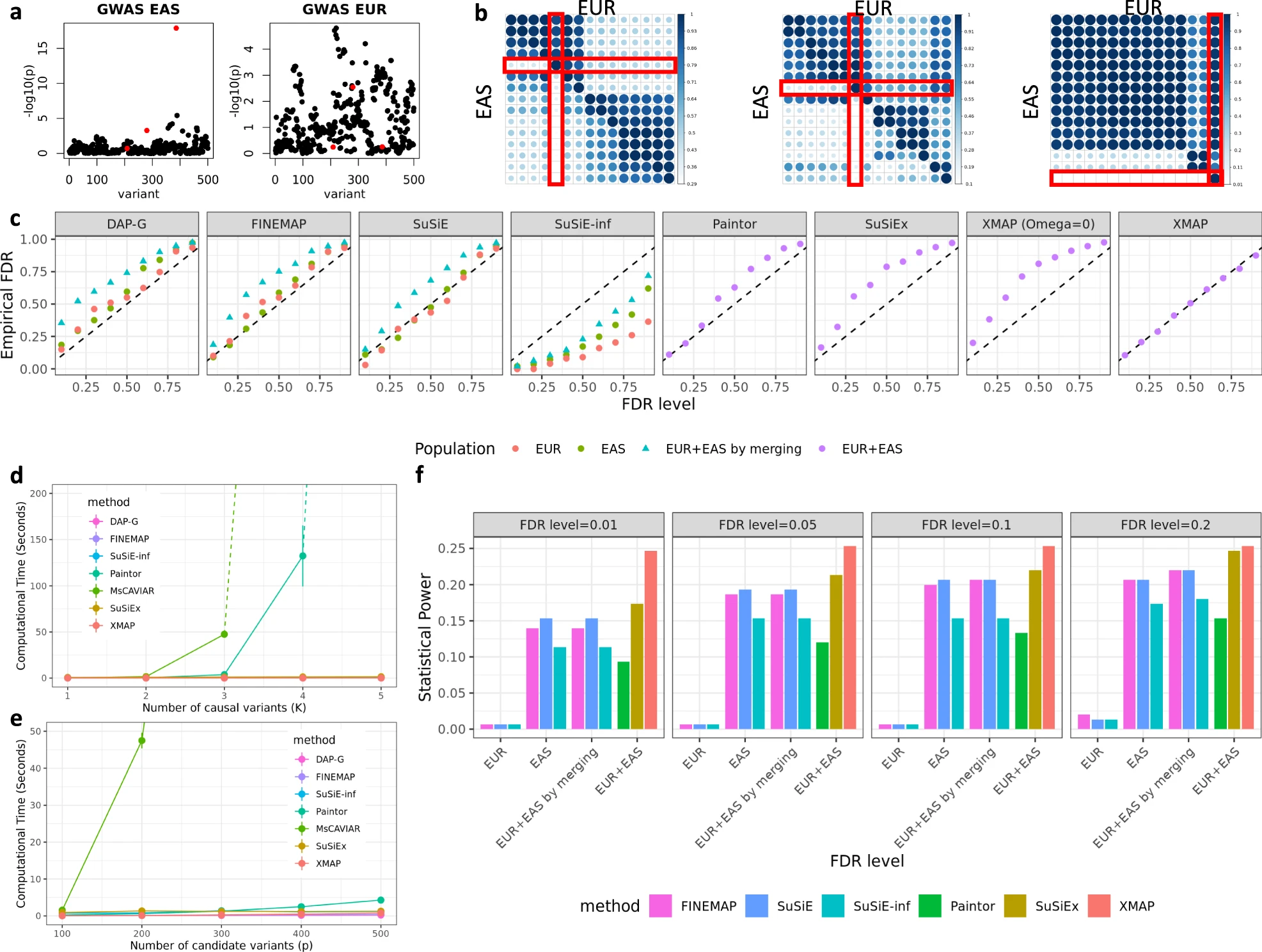
  • Benefit of leveraging genetic diversity: Region in chromosome 22 with p = 500 SNPs. Selected 3 candidate SNPs that: (i) In EUR population in high LD with at least three non-causal SNPs. (ii) In EAS population weakly correlated with non-causal SNPs.
  • Unbalanced populations samples: $n_2 = 20,000$ samples from the EUR population and $n_1$: 5000, 10,000, 15,000, and 20,000 from the EAS population.
  • Reference LD matrices: Used the EUR LD matrix estimated with 337,491 British UKBB samples and estimated the EAS LD matrix with 35,989 EAS samples from the Chinese cohort.
• Scenarios:
  • Scenario 1: Demonstrated the benefit of cross-population fine-mapping by generating GWAS data without confounding bias.
    • Settings:
      • Polygenic effects generated for all 44,728 SNPs in chromosome 22 include the 500-SNPs target region. Total heritability: 5e-3.
      • Heritability of the target SNPs: 50 fold higher than the non-causal SNPs.
      • Effect sizes of the target SNPs are not necessarily the same in the two populations.
      • Genetic correlation between the two populations: 0.8.
      • Standardized $\mathbf{X}$ to have zero mean and unit variance.
      • 50 simulation replicates.
      • Identified causal SNPs by controlling the global FDR.
    • Evaluation: FDR calibration, power, computational efficiency, and the robustness when mis-specifying the genetic effects.

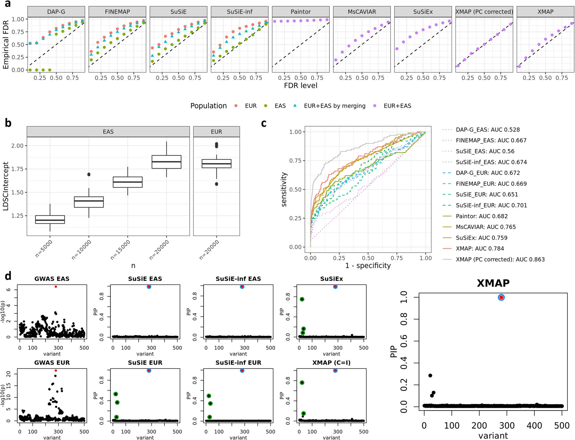
• Scenario 2: Examined the effectiveness of XMAP in correcting confounding bias by simulating GWAS summary data with unadjusted sample structure.
  • Settings: Simulated unadjusted confounding bias with the first principal components from the two populations. Rescaled PC1 to have mean zero and variance 0.05 and PC2 to have mean zero and variance 0.2 which aim to introduce the proper level of inflation in the summary statistics.
    1. Regress phenotype vectors on each SNP excluding the PCs as covariates, representing the scenario with unadjusted confounding bias.
    2. Regress phenotype vectors on each SNP while including the PCs as covariates, representing the scenario with adjusted confounding bias.
  • Conclusion: It is effective to use the inflation constants to correct confounding bias in GWAS.

Real Data Analysis

1. LDL GWASs:
   • Data: GWASs of AFR and EAS (by GLGC) and EUR (by UKBB and GLGC).

   For AFR, we estimated the LD matrices by using 3,072 African individuals from UKBB as reference samples.

   • Confounding bias: The LDSC intercepts estimated from all LDL GWASs were not substantially different from one, suggesting an ignorable confounding bias here.
   • Credibility: Evaluated the replication rate using an independent LDL GWAS from the EUR population.
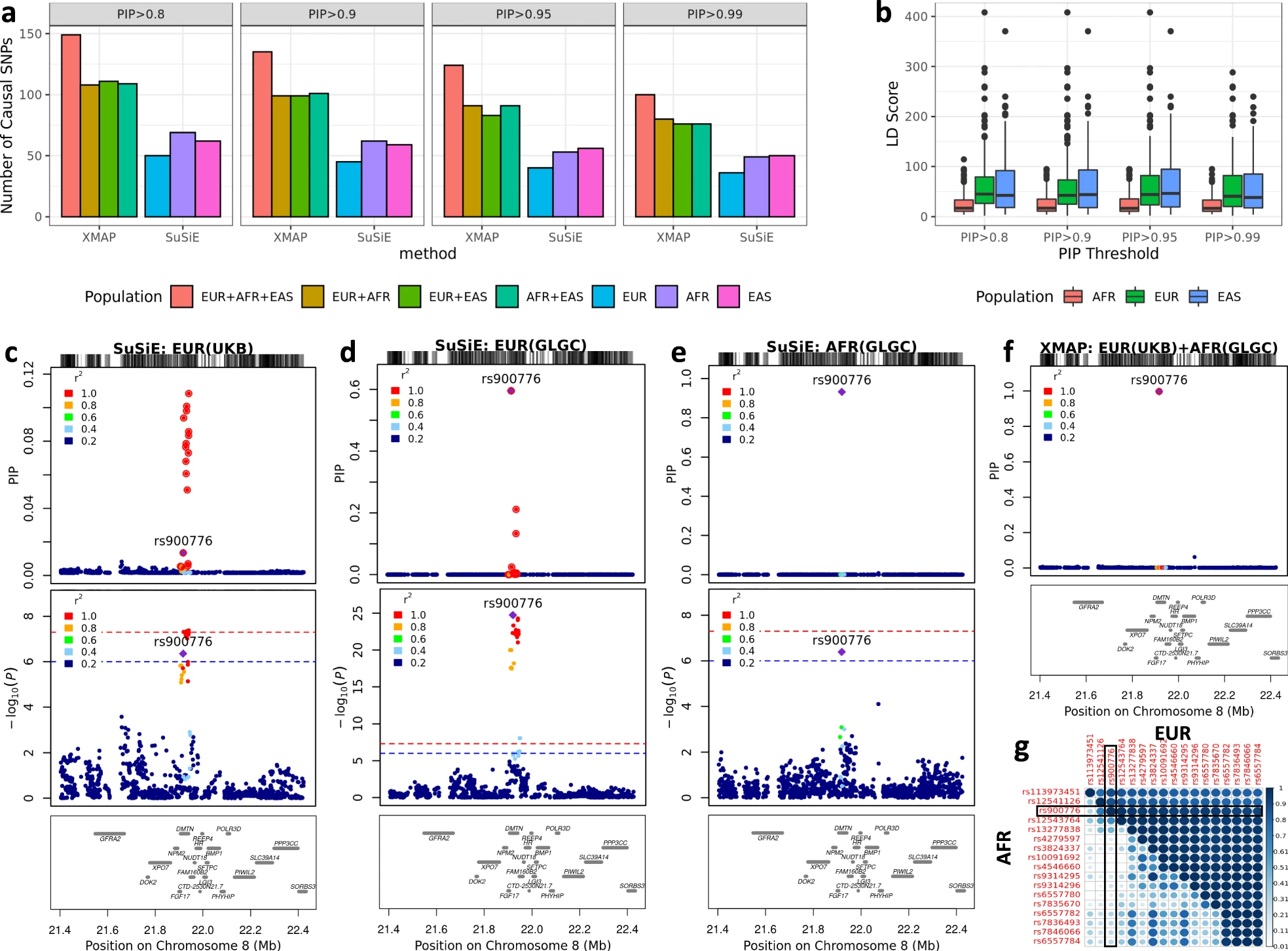
   • Improvement of the power: Use rs900776 as an example to show the improvement of fine-mapping power and resolution by XMAP is owing to leverage the genetic diversity. [should compare the results of XMAP in 3 populations separately and altogether?]

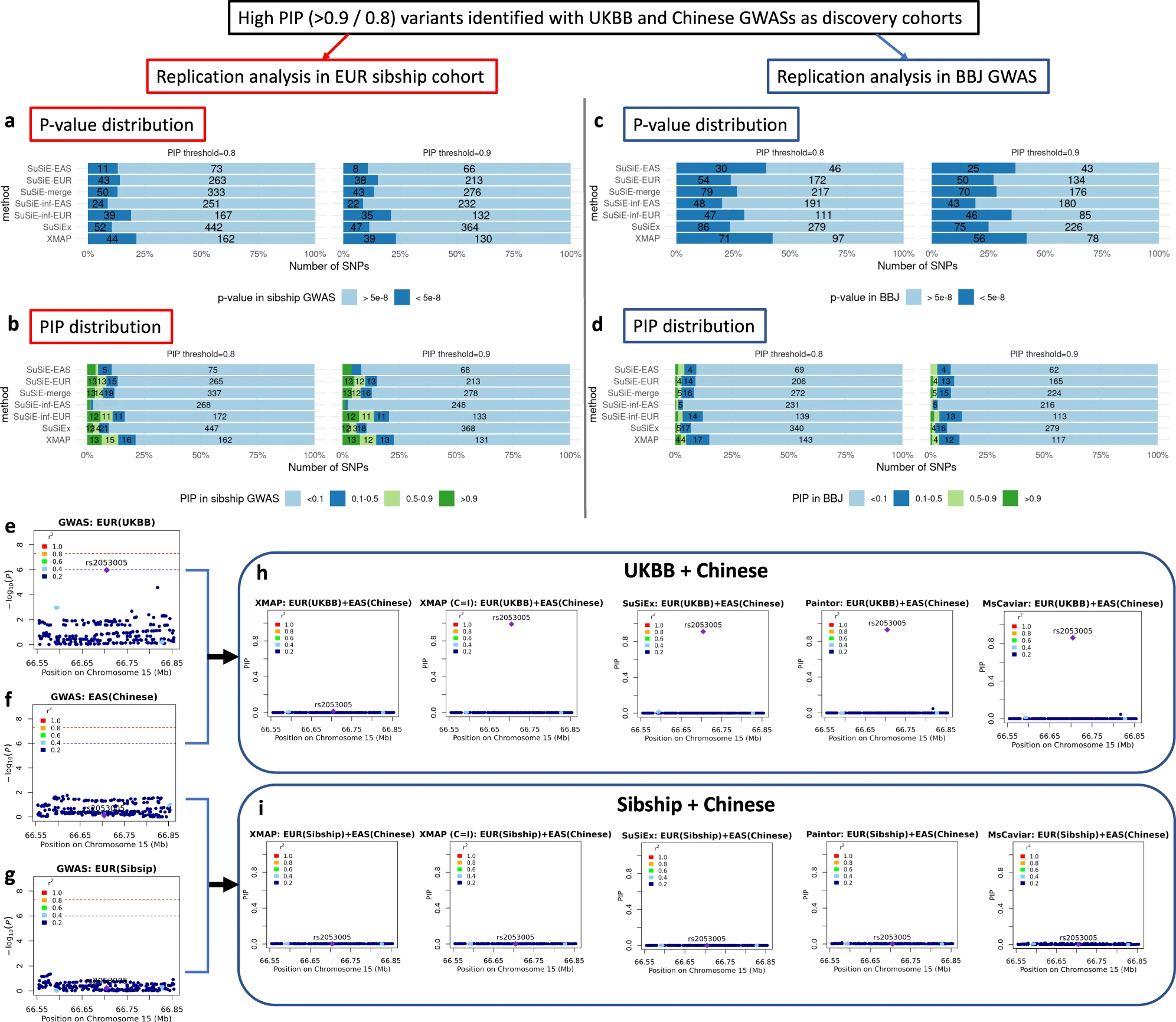
2. Height GWASs: which were well known to be affected by population structure.
   • Aim: Investigate the ability of XMAP in correcting confounding bias and reducing false positive signals.
   • Process: First applied fine-mapping methods to discovery GWAS datasets, and then evaluated the credibility in replication datasets from different population backgrounds.
   • Data: Strong confounding bias: EUR GWAS from UKBB and a Chinese GWAS.
   • Replication data: Ignorable confounding bias: Within-sibship GWAS from European population, which was known to be less confounded by population structure. The GWAS from BBJ cohort from EAS background.
   • Result: Rs2053005 could be a false positive and XMAP was able to exclude this signal by correcting the confounding bias.

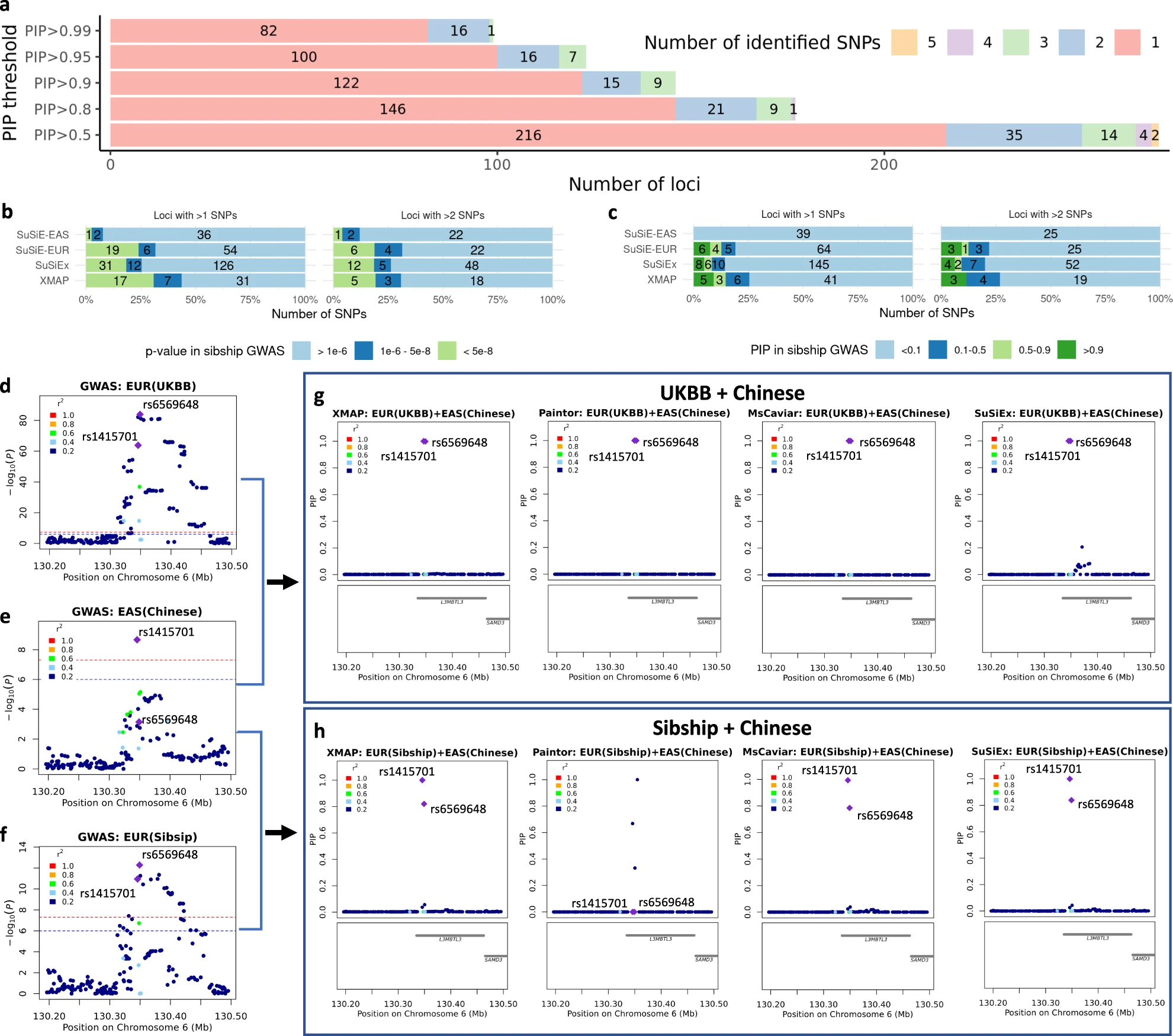
3. Multiple causal signals: XMAP was able to identify multiple causal signals within a locus.
   • Data: Same with 2.
   • Results: XMAP, MsCaviar, and SuSiEx robustly identified multiple causal signals when the sample size decreased. XMAP robust to the choice of $K$ which is max # of causal signals.

4. Single-cell data integration: XMAP results can be effectively integrated with single-cell datasets to identify disease/trait-relevant cells.
   • Data: Blood traits from scATAC-seq dataset that encompasses multiple hematopoietic lineages.
   • Process: ...
   • Result: Better interpretation of risk variants in their relevant cellular context, gaining biological insights into causal mechanisms at single-cell resolution.

Limitations

1. Assumptions: XMAP assumes that the causal variants are shared across populations, which may not be true for some signals (Same as PAINTOR and MsCAVIAR).
2. Disproportionate distribution of causal variants: Causal variants are reported to be distributed disproportionately in the genome, depending on the functional context of the genomic regions.
3. Gene-level effects: Gene-level effects can be more stably shared across populations, as compared to SNP-level effects. Leveraging the genetic diversity at the gene-level for fine-mapping can be an interesting direction.

Reference

Cai M, Wang Z, Xiao J, et al. XMAP: Cross-population fine-mapping by leveraging genetic diversity and accounting for confounding bias[J]. Nature Communications, 2023, 14(1): 6870.

TO-DO

1. In real data's 1.