Running the Tutorial
This tutorial provides a hands-on guide to applying traceCB using a sample dataset (provided as a "toy example") to analyze a single gene. We offer two methods to run this tutorial:
- Google Colab (Recommended): A cloud-based environment requiring no installation.
- Local Execution: Running the tutorial on your own machine.
Consistent Results
Both notebooks use the same public toy inputs. Colab downloads the current default branch; for manuscript reproduction, use a fixed source archive or Git commit and the Python environment in environment.yml. Numerical results can vary across dependency versions.
Option 1: Quick Start with Google Colab
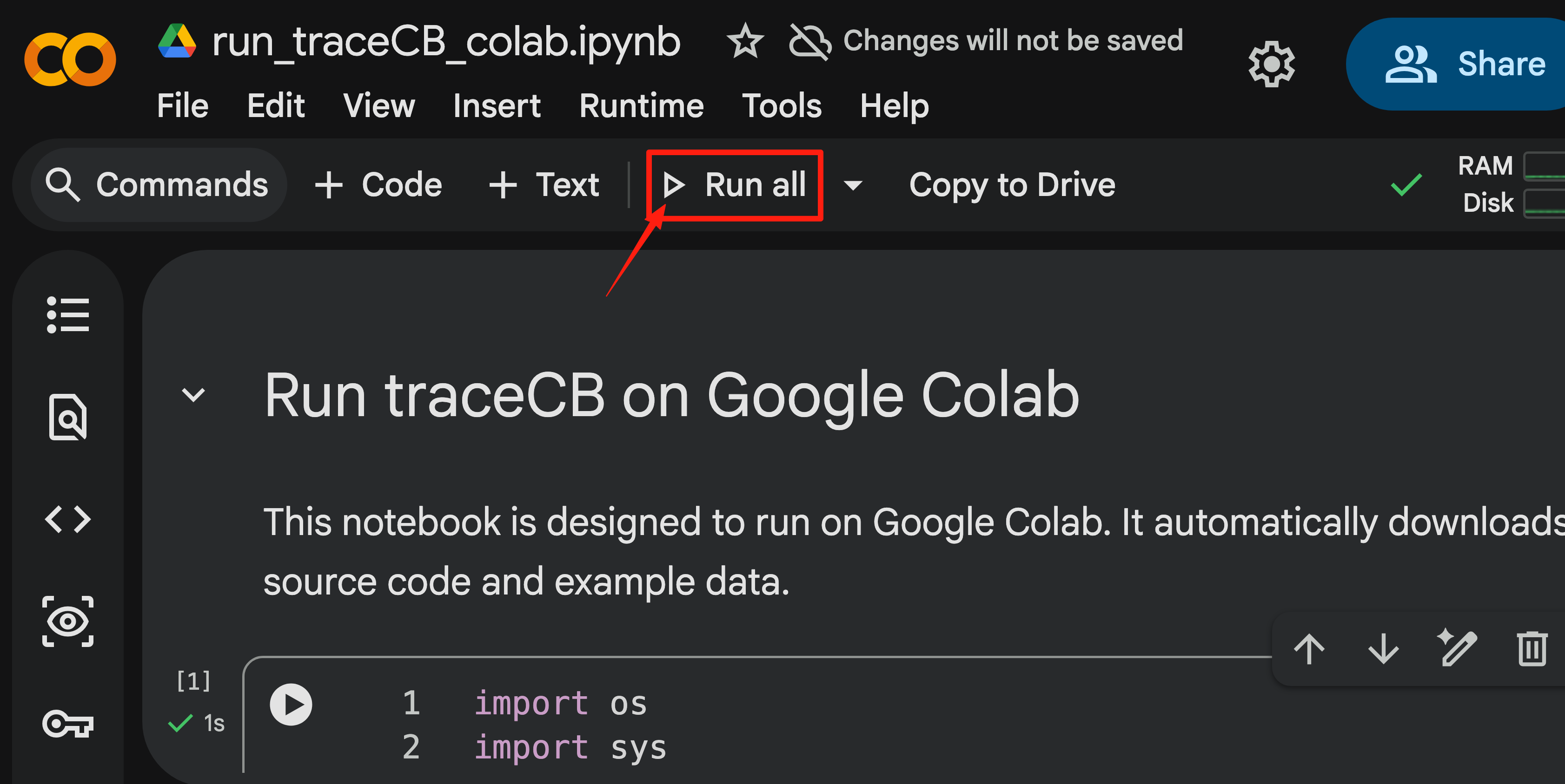
For immediate exploration without configuring a local environment, use our Google Colab notebook. Click the link below to open the tutorial directly in Colab, and use the Run All option to execute the entire notebook to see the results.

Option 2: Local Environment
For researchers preferring a local setup, the tutorial is available as a Jupyter Notebook.
- Install traceCB: Run
pip install -e '.[tutorial]'in the repository root (see the Installation Guide). - Open the Notebook: Navigate to the tutorial notebook at
docs/tutorial/run_traceCB.ipynband open it with Jupyter Notebook or VS Code (or any compatible IDE). - Run Locally: Execute the file to reproduce the analysis.
Run all cells in order. The example aligns 2,072 variants for gene
ENSG00000025708, estimates the cross-population covariance, and compares
summary-statistic, traceC, and traceCB effects. Cell-type proportions in the
input CSV are percentages and are divided by 100 before modeling. If the
bulk-tissue covariance check fails, the tutorial uses the traceC estimates for
the tissue-enhanced output, matching the full-data runner.
Before execution, verify the example inputs from the repository root:
sha256sum --check data/toy_example/SHA256SUMS
The notebook outputs are deliberately cleared in Git. Executing the notebooks creates tables and effective-sample-size summaries locally.